Data and Business Decision Making: Analysis of Employee Data
VerifiedAdded on 2022/11/01
|15
|1220
|381
Project
AI Summary
This assignment is a project analyzing a dataset of young employee information from Tasmania, focusing on the relationships between employee wages and various factors such as education, IQ, work experience, and KW scores. The project involves data cleaning, descriptive statistics, and the use of regression analysis to determine the impact of different variables on wages. Statistical tests, including hypothesis testing and confidence interval calculations, are performed to draw conclusions about the data. The analysis includes scatter plots, histograms, and regression models to assess the significance of different variables. The student also evaluates the goodness of fit for different models, comparing the explanatory power of various factors on employee wages. The project concludes with a discussion of the key findings and their implications for business decision-making.
Running head: DATA AND BUSINESS DECISION MAKING
Data and Business Decision Making
Name of the Student
Name of the University
Course ID
Data and Business Decision Making
Name of the Student
Name of the University
Course ID
Paraphrase This Document
Need a fresh take? Get an instant paraphrase of this document with our AI Paraphraser
1DATA AND BUSINESS DECISION MAKING
Table of Contents
Answer to question 1.......................................................................................................................2
Answer to question 2.......................................................................................................................2
Answer to question 3.......................................................................................................................3
Answer to question 4.1....................................................................................................................5
Answer to question 4.2....................................................................................................................6
Answer to question 4.3....................................................................................................................6
Answer to question 4.4....................................................................................................................7
Answer to question 4.5....................................................................................................................7
Answer to question 5.1....................................................................................................................8
Answer to question 6.1..................................................................................................................10
Answer to question 6.2..................................................................................................................10
Answer to question 6.3..................................................................................................................11
Answer to question 6.4..................................................................................................................11
Answer to question 6.5..................................................................................................................12
Answer to question 6.6..................................................................................................................13
Answer to question 6.7..................................................................................................................13
Reference.......................................................................................................................................14
2DATA AND BUSINESS DECISION MAKING
Answer to question 1
The Final dataset is prepared by removing all the missing observations in order to get
consistent and unbiased results. The final dataset has 111 observations.
Answer to question 2
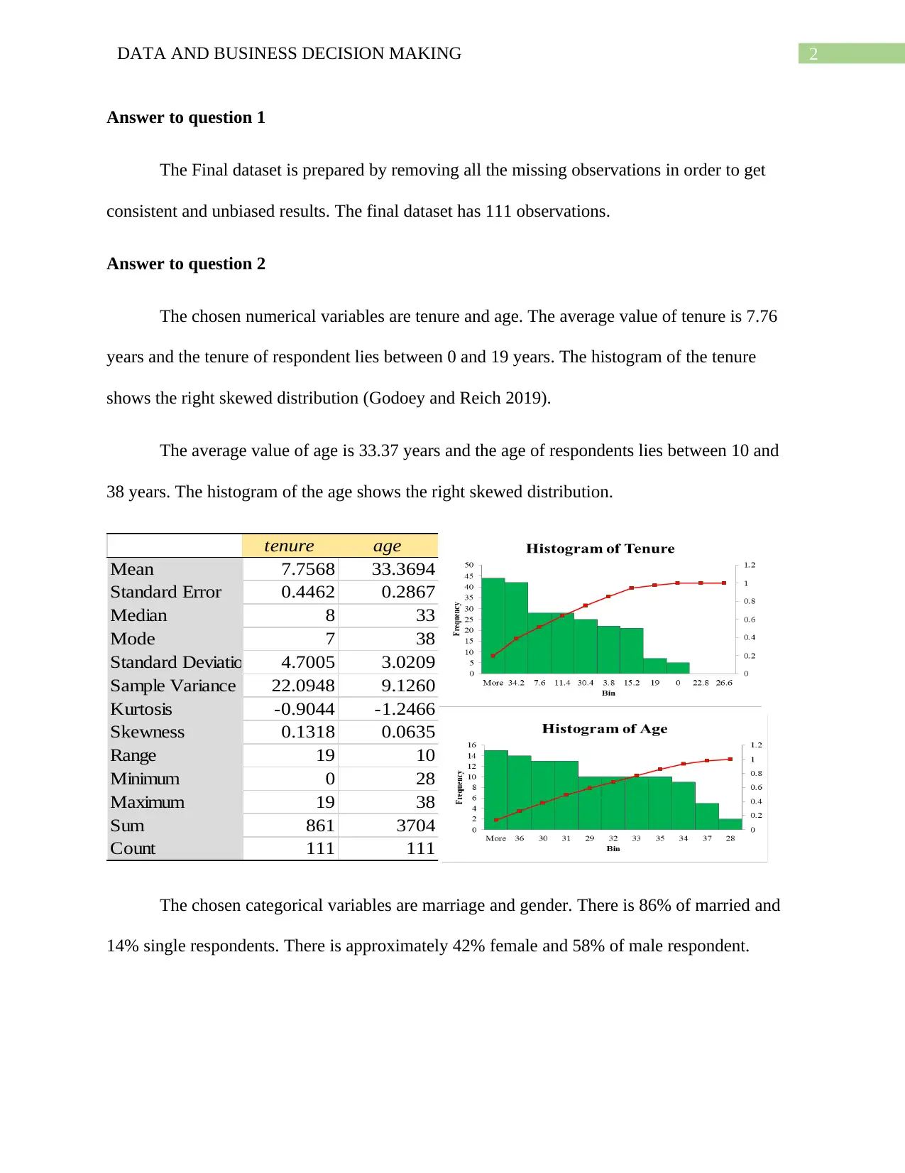
The chosen numerical variables are tenure and age. The average value of tenure is 7.76
years and the tenure of respondent lies between 0 and 19 years. The histogram of the tenure
shows the right skewed distribution (Godoey and Reich 2019).
The average value of age is 33.37 years and the age of respondents lies between 10 and
38 years. The histogram of the age shows the right skewed distribution.
tenure age
Mean 7.7568 33.3694
Standard Error 0.4462 0.2867
Median 8 33
Mode 7 38
Standard Deviation 4.7005 3.0209
Sample Variance 22.0948 9.1260
Kurtosis -0.9044 -1.2466
Skewness 0.1318 0.0635
Range 19 10
Minimum 0 28
Maximum 19 38
Sum 861 3704
Count 111 111
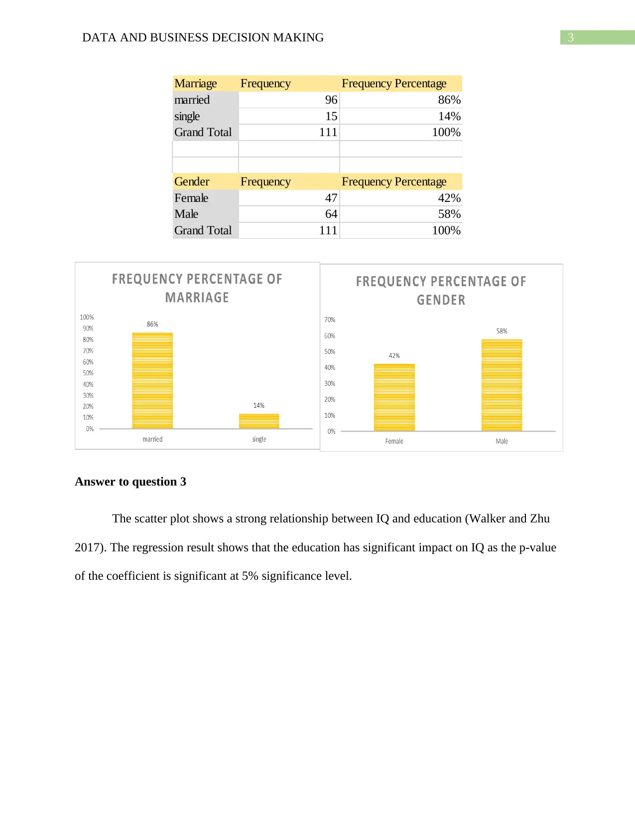
The chosen categorical variables are marriage and gender. There is 86% of married and
14% single respondents. There is approximately 42% female and 58% of male respondent.
Answer to question 1
The Final dataset is prepared by removing all the missing observations in order to get
consistent and unbiased results. The final dataset has 111 observations.
Answer to question 2
The chosen numerical variables are tenure and age. The average value of tenure is 7.76
years and the tenure of respondent lies between 0 and 19 years. The histogram of the tenure
shows the right skewed distribution (Godoey and Reich 2019).
The average value of age is 33.37 years and the age of respondents lies between 10 and
38 years. The histogram of the age shows the right skewed distribution.
tenure age
Mean 7.7568 33.3694
Standard Error 0.4462 0.2867
Median 8 33
Mode 7 38
Standard Deviation 4.7005 3.0209
Sample Variance 22.0948 9.1260
Kurtosis -0.9044 -1.2466
Skewness 0.1318 0.0635
Range 19 10
Minimum 0 28
Maximum 19 38
Sum 861 3704
Count 111 111
The chosen categorical variables are marriage and gender. There is 86% of married and
14% single respondents. There is approximately 42% female and 58% of male respondent.
⊘ This is a preview!⊘
Do you want full access?
Subscribe today to unlock all pages.
Trusted by 1+ million students worldwide
3DATA AND BUSINESS DECISION MAKING
Marriage Frequency Frequency Percentage
married 96 86%
single 15 14%
Grand Total 111 100%
Gender Frequency Frequency Percentage
Female 47 42%
Male 64 58%
Grand Total 111 100%
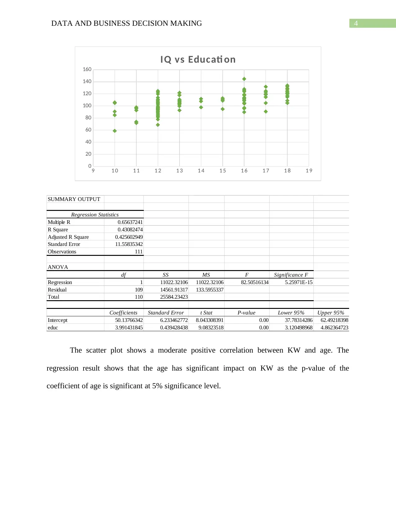
Answer to question 3
The scatter plot shows a strong relationship between IQ and education (Walker and Zhu
2017). The regression result shows that the education has significant impact on IQ as the p-value
of the coefficient is significant at 5% significance level.
Marriage Frequency Frequency Percentage
married 96 86%
single 15 14%
Grand Total 111 100%
Gender Frequency Frequency Percentage
Female 47 42%
Male 64 58%
Grand Total 111 100%
Answer to question 3
The scatter plot shows a strong relationship between IQ and education (Walker and Zhu
2017). The regression result shows that the education has significant impact on IQ as the p-value
of the coefficient is significant at 5% significance level.
Paraphrase This Document
Need a fresh take? Get an instant paraphrase of this document with our AI Paraphraser
4DATA AND BUSINESS DECISION MAKING
9 1 0 1 1 1 2 1 3 1 4 1 5 1 6 1 7 1 8 1 9
0
20
40
60
80
100
120
140
160
IQ vs Educati on
SUMMARY OUTPUT
Regression Statistics
Multiple R 0.65637241
R Square 0.43082474
Adjusted R Square 0.425602949
Standard Error 11.55835342
Observations 111
ANOVA
df SS MS F Significance F
Regression 1 11022.32106 11022.32106 82.50516134 5.25971E-15
Residual 109 14561.91317 133.5955337
Total 110 25584.23423
Coefficients Standard Error t Stat P-value Lower 95% Upper 95%
Intercept 50.13766342 6.233462772 8.043308391 0.00 37.78314286 62.49218398
educ 3.991431845 0.439428438 9.08323518 0.00 3.120498968 4.862364723
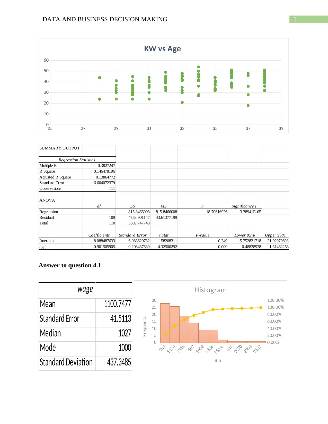
The scatter plot shows a moderate positive correlation between KW and age. The
regression result shows that the age has significant impact on KW as the p-value of the
coefficient of age is significant at 5% significance level.
9 1 0 1 1 1 2 1 3 1 4 1 5 1 6 1 7 1 8 1 9
0
20
40
60
80
100
120
140
160
IQ vs Educati on
SUMMARY OUTPUT
Regression Statistics
Multiple R 0.65637241
R Square 0.43082474
Adjusted R Square 0.425602949
Standard Error 11.55835342
Observations 111
ANOVA
df SS MS F Significance F
Regression 1 11022.32106 11022.32106 82.50516134 5.25971E-15
Residual 109 14561.91317 133.5955337
Total 110 25584.23423
Coefficients Standard Error t Stat P-value Lower 95% Upper 95%
Intercept 50.13766342 6.233462772 8.043308391 0.00 37.78314286 62.49218398
educ 3.991431845 0.439428438 9.08323518 0.00 3.120498968 4.862364723
The scatter plot shows a moderate positive correlation between KW and age. The
regression result shows that the age has significant impact on KW as the p-value of the
coefficient of age is significant at 5% significance level.
5DATA AND BUSINESS DECISION MAKING
25 27 29 31 33 35 37 39
0
10
20
30
40
50
60
KW vs Age
SUMMARY OUTPUT
Regression Statistics
Multiple R 0.3827247
R Square 0.146478196
Adjusted R Square 0.13864772
Standard Error 6.604072379
Observations 111
ANOVA
df SS MS F Significance F
Regression 1 815.8466008 815.8466008 18.70616926 3.38941E-05
Residual 109 4753.901147 43.61377199
Total 110 5569.747748
Coefficients Standard Error t Stat P-value Lower 95% Upper 95%
Intercept 8.088487633 6.983620782 1.158208311 0.249 -5.752821718 21.92979698
age 0.901505905 0.208437639 4.32506292 0.000 0.48838928 1.31462253
Answer to question 4.1
wage
Mean 1100.7477
Standard Error 41.5113
Median 1027
Mode 1000
Standard Deviation 437.3485
901
1134
1368
667
1602
1836
More
433
2070
2303
2537
0
5
10
15
20
25
30
0.00%
20.00%
40.00%
60.00%
80.00%
100.00%
120.00%
Histogram
Bin
Frequency
⊘ This is a preview!⊘
Do you want full access?
Subscribe today to unlock all pages.
Trusted by 1+ million students worldwide
6DATA AND BUSINESS DECISION MAKING
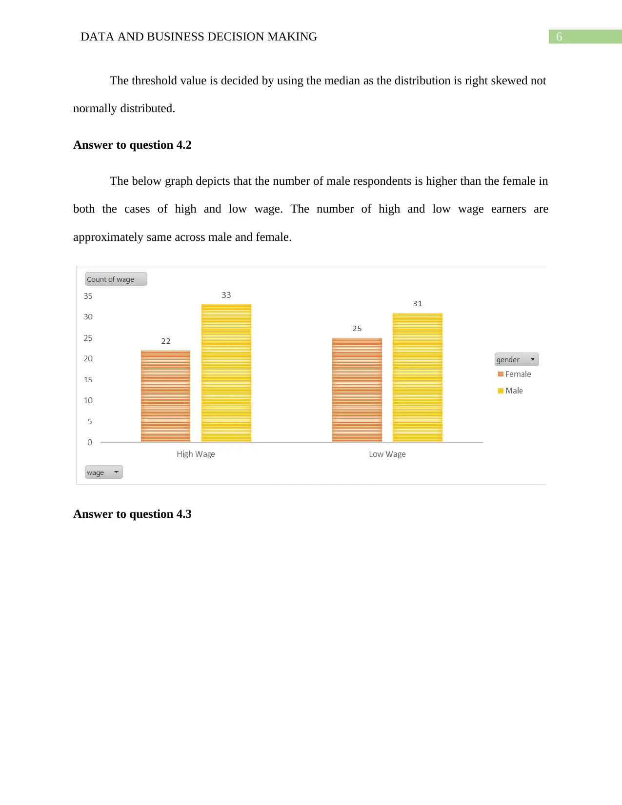
The threshold value is decided by using the median as the distribution is right skewed not
normally distributed.
Answer to question 4.2
The below graph depicts that the number of male respondents is higher than the female in
both the cases of high and low wage. The number of high and low wage earners are
approximately same across male and female.
Answer to question 4.3
Paraphrase This Document
Need a fresh take? Get an instant paraphrase of this document with our AI Paraphraser
7DATA AND BUSINESS DECISION MAKING
Female Male Grand Total
High Wage 22 33 55
Low Wage 25 31 56
Total 47 64 111
Female Male Grand Total
High Wage 0.198 0.297 0.495
Low Wage 0.225 0.279 0.505
Total 0.423 0.577 1.000
Female Male Grand Total
High Wage 0.468 0.516 0.495
Low Wage 0.532 0.484 0.505
Total 1.000 1.000 1.000
Gender
Wage
Joint Probability
Wage
Gender
Marginal Probability
Gender
Wage
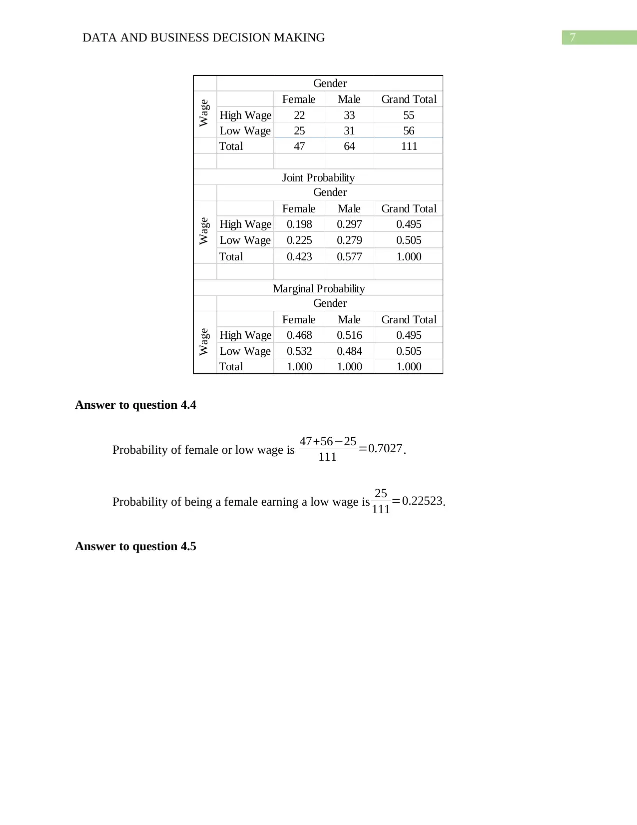
Answer to question 4.4
Probability of female or low wage is 47+56−25
111 =0.7027.
Probability of being a female earning a low wage is 25
111=0.22523.
Answer to question 4.5
Female Male Grand Total
High Wage 22 33 55
Low Wage 25 31 56
Total 47 64 111
Female Male Grand Total
High Wage 0.198 0.297 0.495
Low Wage 0.225 0.279 0.505
Total 0.423 0.577 1.000
Female Male Grand Total
High Wage 0.468 0.516 0.495
Low Wage 0.532 0.484 0.505
Total 1.000 1.000 1.000
Gender
Wage
Joint Probability
Wage
Gender
Marginal Probability
Gender
Wage
Answer to question 4.4
Probability of female or low wage is 47+56−25
111 =0.7027.
Probability of being a female earning a low wage is 25
111=0.22523.
Answer to question 4.5
8DATA AND BUSINESS DECISION MAKING
Female Male Grand Total
High Wage 22 33 55
Low Wage 25 31 56
Total 47 64 111
Female Male Grand Total
High Wage 23.288 31.712 55
Low Wage 23.712 32.288 56
Total 47 64 111
Female Male Grand Total
High Wage 0.071 0.052 0.124
Low Wage 0.070 0.051 0.121
Total 0.141 0.104 0.245
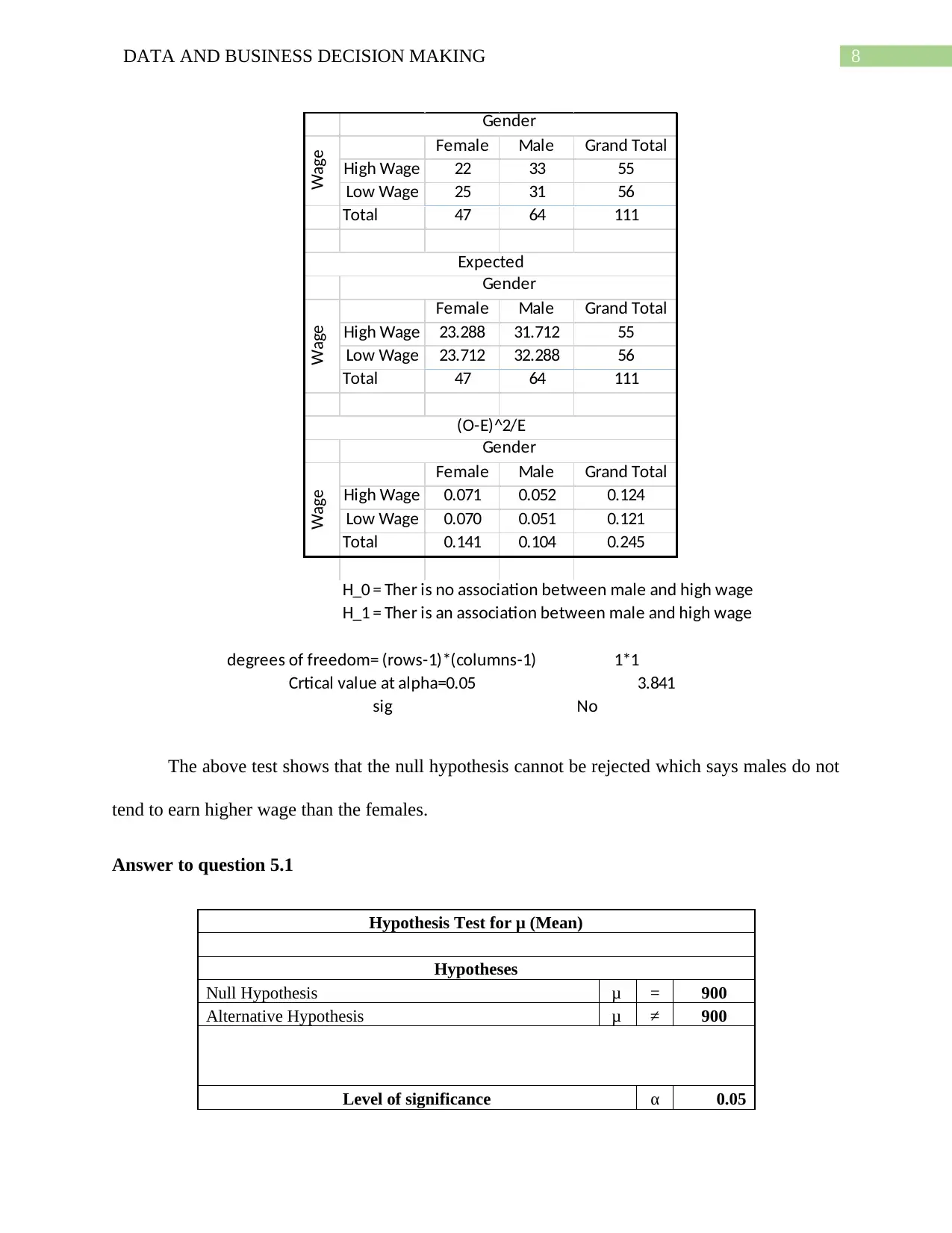
H_0 = Ther is no association between male and high wage
H_1 = Ther is an association between male and high wage
degrees of freedom= (rows-1)*(columns-1) 1*1
Crtical value at alpha=0.05 3.841
sig No
Gender
Wage
Expected
Gender
Wage
(O-E)^2/E
Gender
Wage
The above test shows that the null hypothesis cannot be rejected which says males do not
tend to earn higher wage than the females.
Answer to question 5.1
Hypothesis Test for μ (Mean)
Hypotheses
Null Hypothesis μ = 900
Alternative Hypothesis μ ≠ 900
Level of significance α 0.05
Female Male Grand Total
High Wage 22 33 55
Low Wage 25 31 56
Total 47 64 111
Female Male Grand Total
High Wage 23.288 31.712 55
Low Wage 23.712 32.288 56
Total 47 64 111
Female Male Grand Total
High Wage 0.071 0.052 0.124
Low Wage 0.070 0.051 0.121
Total 0.141 0.104 0.245
H_0 = Ther is no association between male and high wage
H_1 = Ther is an association between male and high wage
degrees of freedom= (rows-1)*(columns-1) 1*1
Crtical value at alpha=0.05 3.841
sig No
Gender
Wage
Expected
Gender
Wage
(O-E)^2/E
Gender
Wage
The above test shows that the null hypothesis cannot be rejected which says males do not
tend to earn higher wage than the females.
Answer to question 5.1
Hypothesis Test for μ (Mean)
Hypotheses
Null Hypothesis μ = 900
Alternative Hypothesis μ ≠ 900
Level of significance α 0.05
⊘ This is a preview!⊘
Do you want full access?
Subscribe today to unlock all pages.
Trusted by 1+ million students worldwide
9DATA AND BUSINESS DECISION MAKING
Critical Value (s) 1.9600
Population Standard Deviation 437.3485
Sample Data
Sample Mean 1100.748
Sample Size 111
Standard Error of the Mean 41.51
Z Sample Statistic 4.835981
p-value 0.000003
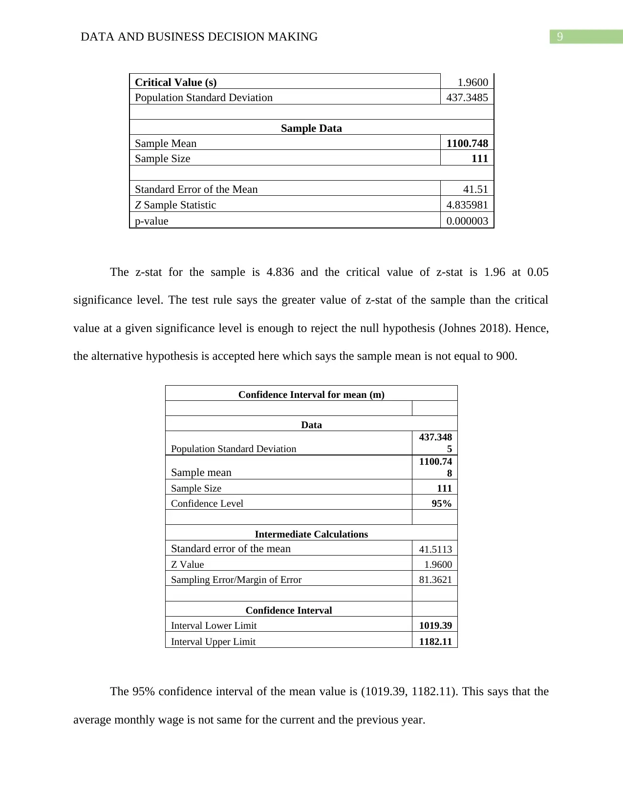
The z-stat for the sample is 4.836 and the critical value of z-stat is 1.96 at 0.05
significance level. The test rule says the greater value of z-stat of the sample than the critical
value at a given significance level is enough to reject the null hypothesis (Johnes 2018). Hence,
the alternative hypothesis is accepted here which says the sample mean is not equal to 900.
Confidence Interval for mean (m)
Data
Population Standard Deviation
437.348
5
Sample mean
1100.74
8
Sample Size 111
Confidence Level 95%
Intermediate Calculations
Standard error of the mean 41.5113
Z Value 1.9600
Sampling Error/Margin of Error 81.3621
Confidence Interval
Interval Lower Limit 1019.39
Interval Upper Limit 1182.11
The 95% confidence interval of the mean value is (1019.39, 1182.11). This says that the
average monthly wage is not same for the current and the previous year.
Critical Value (s) 1.9600
Population Standard Deviation 437.3485
Sample Data
Sample Mean 1100.748
Sample Size 111
Standard Error of the Mean 41.51
Z Sample Statistic 4.835981
p-value 0.000003
The z-stat for the sample is 4.836 and the critical value of z-stat is 1.96 at 0.05
significance level. The test rule says the greater value of z-stat of the sample than the critical
value at a given significance level is enough to reject the null hypothesis (Johnes 2018). Hence,
the alternative hypothesis is accepted here which says the sample mean is not equal to 900.
Confidence Interval for mean (m)
Data
Population Standard Deviation
437.348
5
Sample mean
1100.74
8
Sample Size 111
Confidence Level 95%
Intermediate Calculations
Standard error of the mean 41.5113
Z Value 1.9600
Sampling Error/Margin of Error 81.3621
Confidence Interval
Interval Lower Limit 1019.39
Interval Upper Limit 1182.11
The 95% confidence interval of the mean value is (1019.39, 1182.11). This says that the
average monthly wage is not same for the current and the previous year.
Paraphrase This Document
Need a fresh take? Get an instant paraphrase of this document with our AI Paraphraser
10DATA AND BUSINESS DECISION MAKING
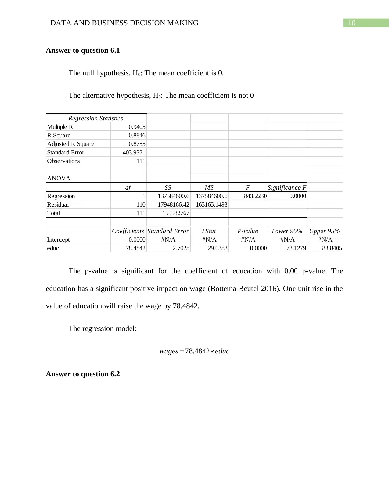
Answer to question 6.1
The null hypothesis, H0: The mean coefficient is 0.
The alternative hypothesis, H0: The mean coefficient is not 0
Regression Statistics
Multiple R 0.9405
R Square 0.8846
Adjusted R Square 0.8755
Standard Error 403.9371
Observations 111
ANOVA
df SS MS F Significance F
Regression 1 137584600.6 137584600.6 843.2230 0.0000
Residual 110 17948166.42 163165.1493
Total 111 155532767
Coefficients Standard Error t Stat P-value Lower 95% Upper 95%
Intercept 0.0000 #N/A #N/A #N/A #N/A #N/A
educ 78.4842 2.7028 29.0383 0.0000 73.1279 83.8405
The p-value is significant for the coefficient of education with 0.00 p-value. The
education has a significant positive impact on wage (Bottema‐Beutel 2016). One unit rise in the
value of education will raise the wage by 78.4842.
The regression model:
wages=78.4842∗educ
Answer to question 6.2
11DATA AND BUSINESS DECISION MAKING
Regression Statistics
Multiple R 0.9414
R Square 0.8861
Adjusted R Square 0.8771
Standard Error 401.2297
Observations 111
ANOVA
df SS MS F Significance F
Regression 1 137824386.7 137824386.69 856.13 0.00
Residual 110 17708380.31 160985.28
Total 111 155532767
Coefficients Standard Error t Stat P-value Lower 95% Upper 95%
Intercept 0 #N/A #N/A #N/A #N/A #N/A
IQ 10.4182 0.3561 29.2597 0.0000 9.7126 11.1238
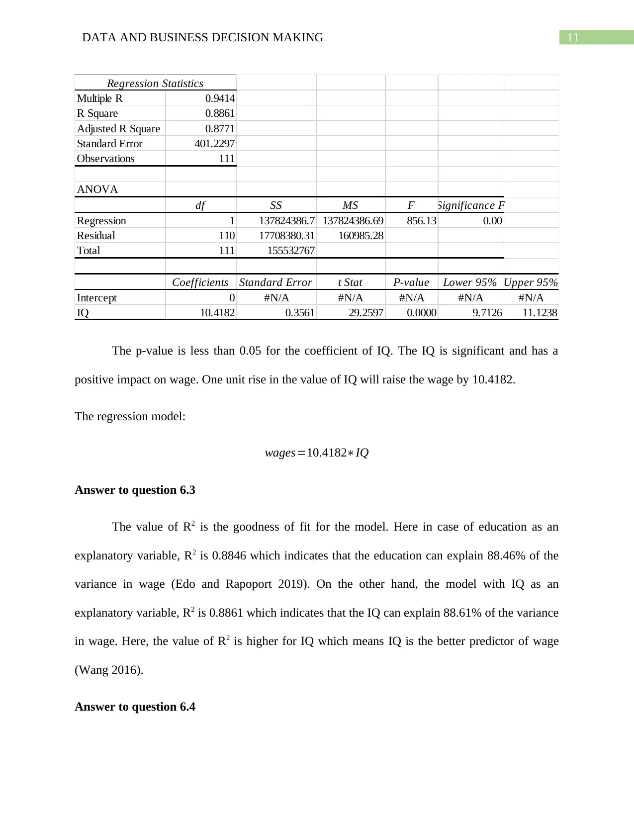
The p-value is less than 0.05 for the coefficient of IQ. The IQ is significant and has a
positive impact on wage. One unit rise in the value of IQ will raise the wage by 10.4182.
The regression model:
wages=10.4182∗IQ
Answer to question 6.3
The value of R2 is the goodness of fit for the model. Here in case of education as an
explanatory variable, R2 is 0.8846 which indicates that the education can explain 88.46% of the
variance in wage (Edo and Rapoport 2019). On the other hand, the model with IQ as an
explanatory variable, R2 is 0.8861 which indicates that the IQ can explain 88.61% of the variance
in wage. Here, the value of R2 is higher for IQ which means IQ is the better predictor of wage
(Wang 2016).
Answer to question 6.4
Regression Statistics
Multiple R 0.9414
R Square 0.8861
Adjusted R Square 0.8771
Standard Error 401.2297
Observations 111
ANOVA
df SS MS F Significance F
Regression 1 137824386.7 137824386.69 856.13 0.00
Residual 110 17708380.31 160985.28
Total 111 155532767
Coefficients Standard Error t Stat P-value Lower 95% Upper 95%
Intercept 0 #N/A #N/A #N/A #N/A #N/A
IQ 10.4182 0.3561 29.2597 0.0000 9.7126 11.1238
The p-value is less than 0.05 for the coefficient of IQ. The IQ is significant and has a
positive impact on wage. One unit rise in the value of IQ will raise the wage by 10.4182.
The regression model:
wages=10.4182∗IQ
Answer to question 6.3
The value of R2 is the goodness of fit for the model. Here in case of education as an
explanatory variable, R2 is 0.8846 which indicates that the education can explain 88.46% of the
variance in wage (Edo and Rapoport 2019). On the other hand, the model with IQ as an
explanatory variable, R2 is 0.8861 which indicates that the IQ can explain 88.61% of the variance
in wage. Here, the value of R2 is higher for IQ which means IQ is the better predictor of wage
(Wang 2016).
Answer to question 6.4
⊘ This is a preview!⊘
Do you want full access?
Subscribe today to unlock all pages.
Trusted by 1+ million students worldwide
1 out of 15