HI6007 Statistics Assignment: Data Analysis, Regression, Holmes

This assignment solution provides a comprehensive analysis of statistical data, focusing on regression modeling. It covers various aspects, including data collection methods, sampling techniques like stratified random sampling, and the identification of independent and dependent variables. The solution addresses potential issues in data collection, examines frequency distributions, and interprets scatter plots. It further delves into regression analysis, providing the equation of the estimated fitting line, numerical summaries, and correlation coefficients. The assignment also includes a detailed analysis of a multiple regression model, interpreting standard error, R-squared values, and hypothesis testing, ultimately determining the significance of various factors in the model. This resource is helpful for students seeking to understand and apply statistical techniques, with Desklib providing additional support through access to past papers and solved assignments.

STATISTICS
Student ID:
[Pick the date]

Question 1
a) An online survey method could be used for data collection considering the fact that the
underlying questions are straight forward and also obtaining the selected random sample
through face to face or other means may be difficult. It would make sense to have a higher
sample fill in the online survey in relation to the preparation hours and the marks scored and
then through technology enabled tools, the requisite sample of 100 can be obtained (Hillier,
2016).
b) The requisite sampling method which would be used to select the sample would be
stratified random sampling. This would be preferred over simple random sampling so as to
ensure that key attributes such as gender, educational background, country of origin and other
aspects could be taken care of and a sample that is representative of the population may be
obtianed. Using a simple random sample instead could lead to the sample being non-
representative as certain attributes may be over-represented while other under-represented
(Flick, 2015).
c) The independent variable is the amount of preparation time that each student spends while
the dependent variable is the number of marks scored in exam. This is because typcially the
marks scored would be dependent on the amount of preparation that is done by the students
and not the other way around. Both the given data are numerical in nature and the
measurement scale would be ratio considering the absolute zero can be defined for both
variables (Eriksson & Kovalainen, 2015).
d) Potential issues that may be faced with regards to collection of data are highlighted below
(Medhi, 2016).
 It is possible that students may not have a fair estiamte of the exact preparation time
and also the time frame over which the same has to be stated. For instance, should be
include 24 hours before the exam or a week or a month before the exam.
 Also, it might be possible that students may tend to overestiamte and underestiamte
their study hours. For instance, students with good marks are likely to reportn higher
study hours as compared to those who have lower marks in exam.
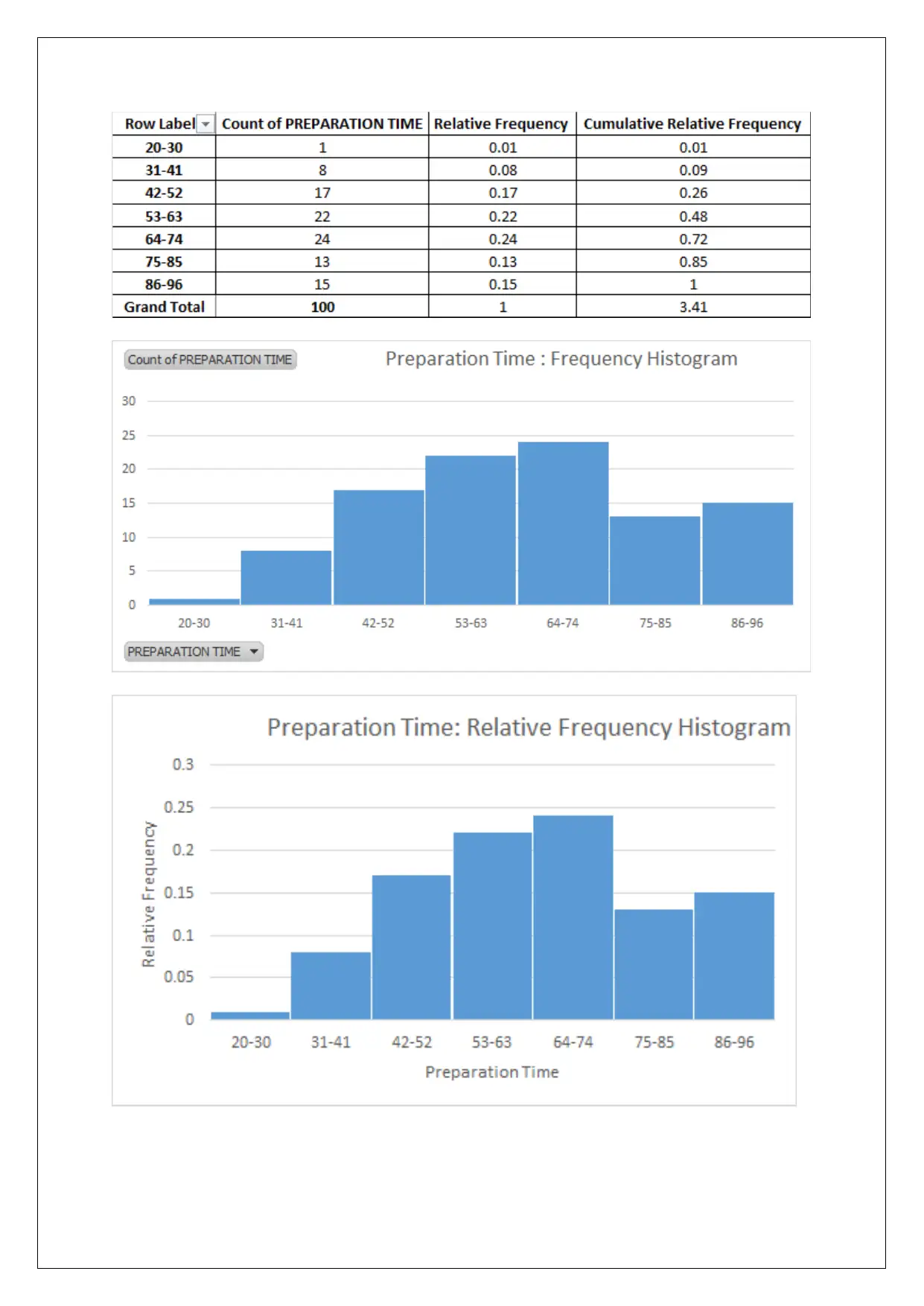
e) The frequency distribution of preparation time is indicated below.

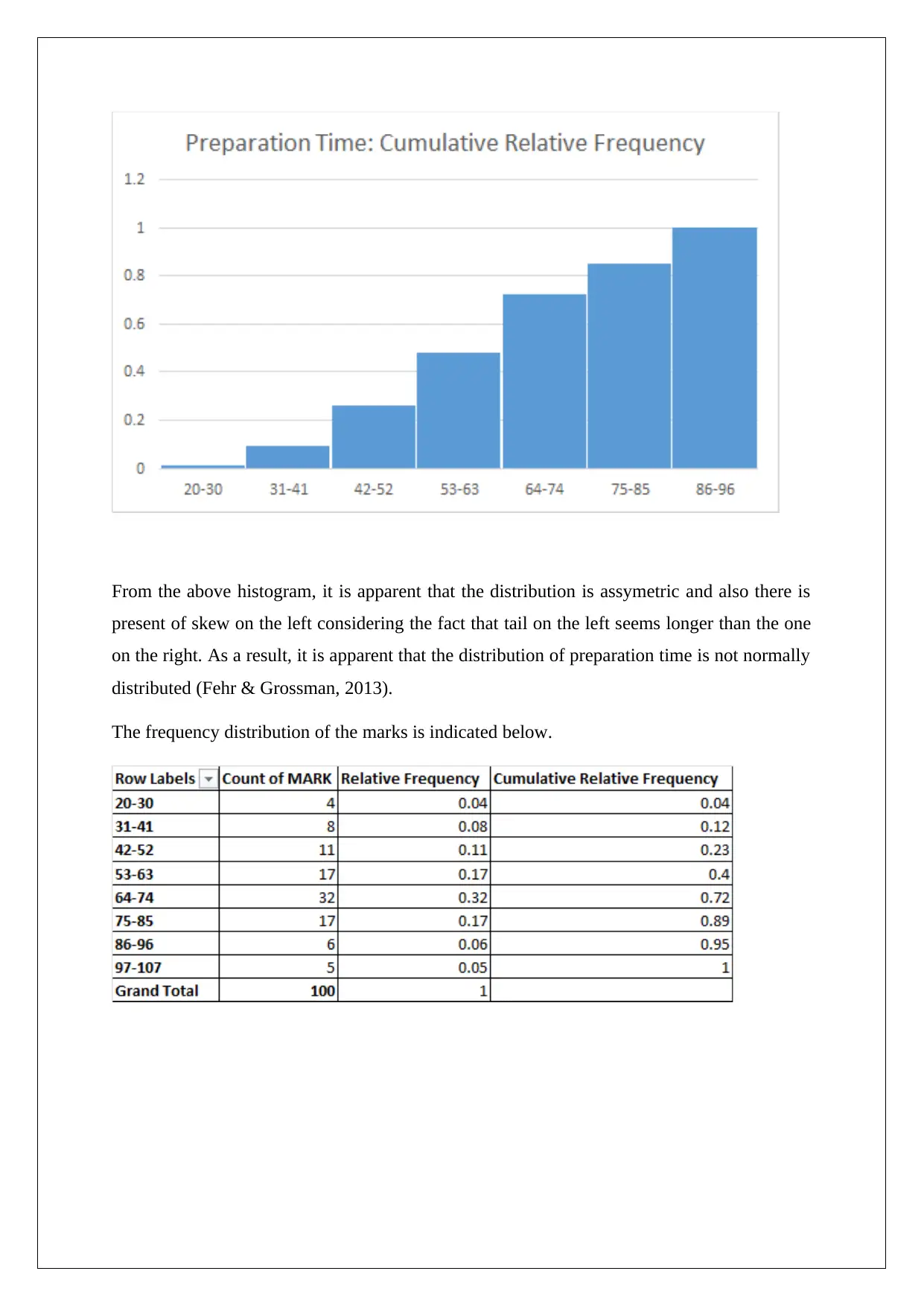
From the above histogram, it is apparent that the distribution is assymetric and also there is
present of skew on the left considering the fact that tail on the left seems longer than the one
on the right. As a result, it is apparent that the distribution of preparation time is not normally
distributed (Fehr & Grossman, 2013).
The frequency distribution of the marks is indicated below.

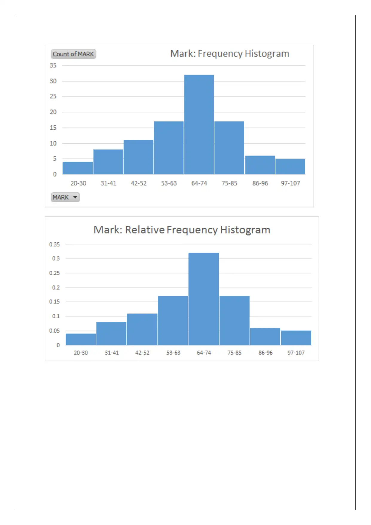
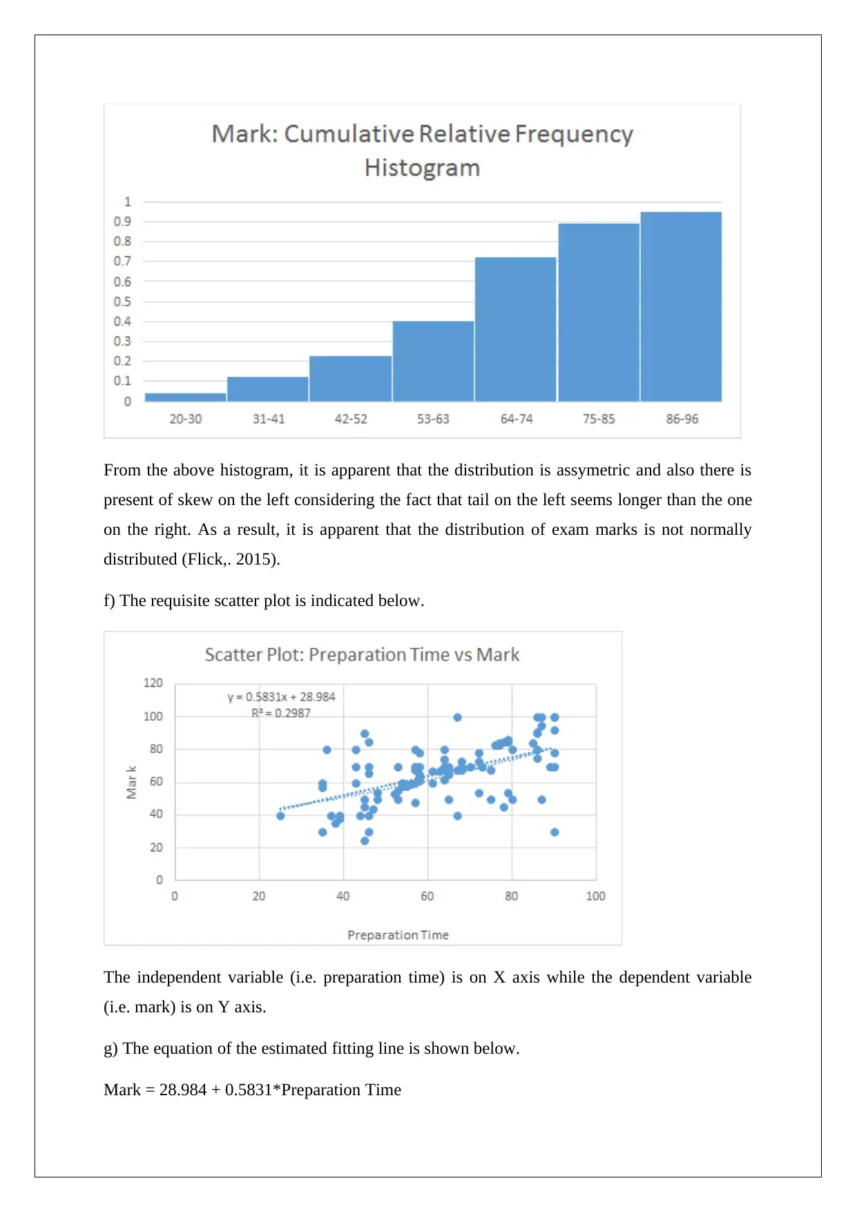
From the above histogram, it is apparent that the distribution is assymetric and also there is
present of skew on the left considering the fact that tail on the left seems longer than the one
on the right. As a result, it is apparent that the distribution of exam marks is not normally
distributed (Flick,. 2015).
f) The requisite scatter plot is indicated below.
The independent variable (i.e. preparation time) is on X axis while the dependent variable
(i.e. mark) is on Y axis.
g) The equation of the estimated fitting line is shown below.
Mark = 28.984 + 0.5831*Preparation Time

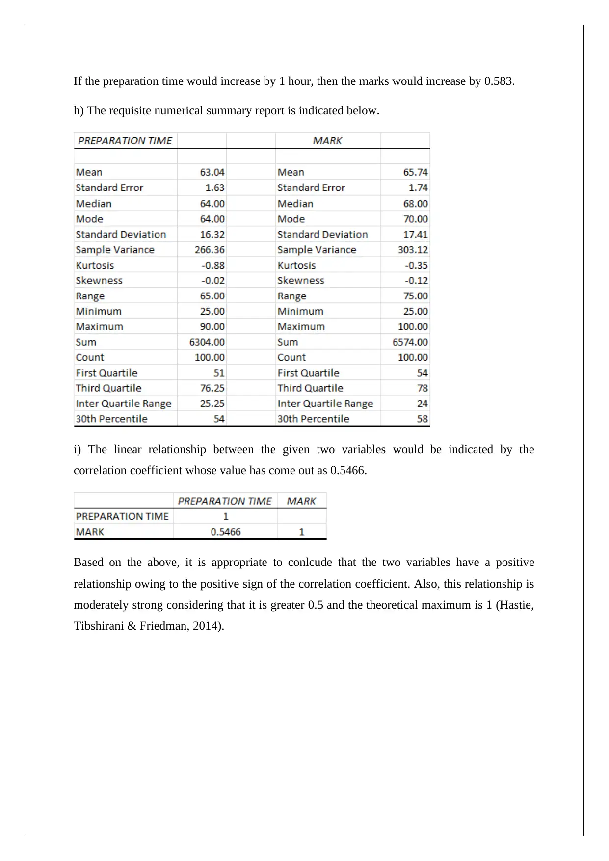
If the preparation time would increase by 1 hour, then the marks would increase by 0.583.
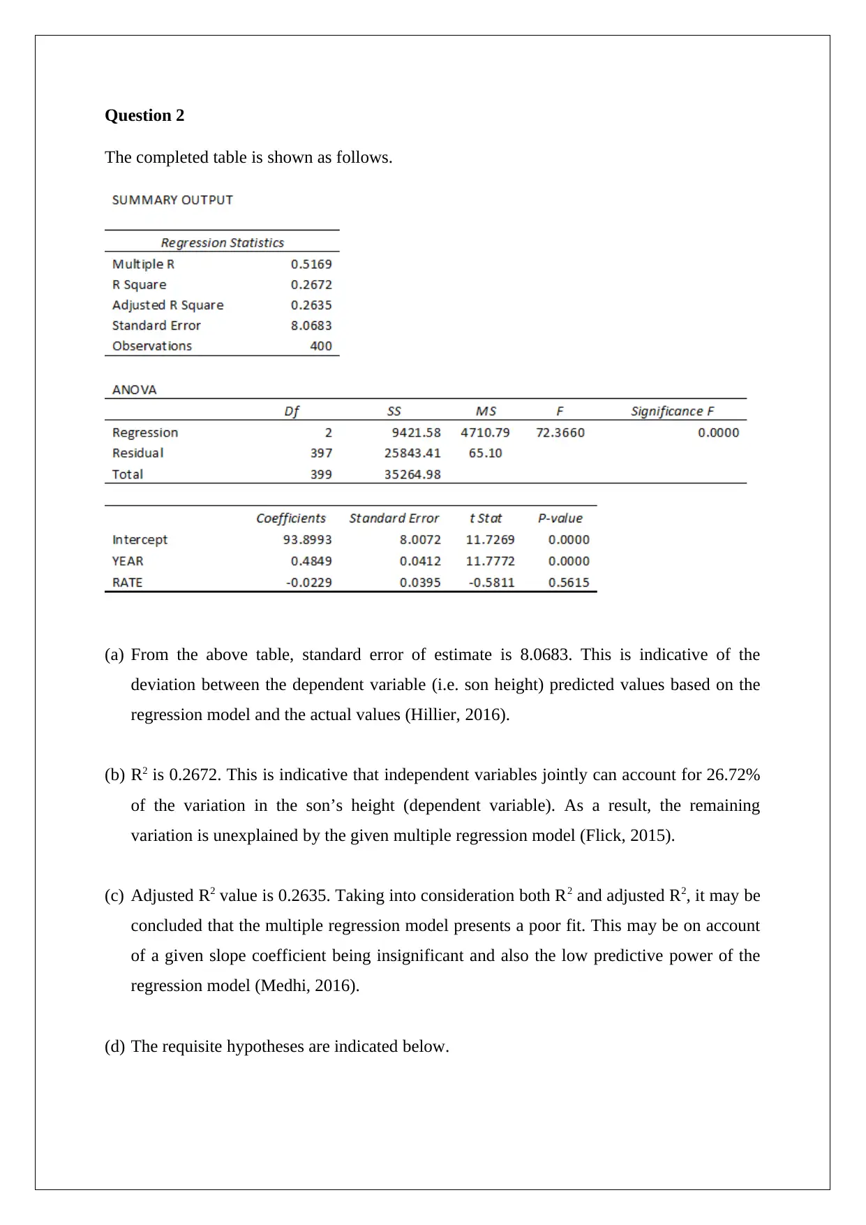
h) The requisite numerical summary report is indicated below.
i) The linear relationship between the given two variables would be indicated by the
correlation coefficient whose value has come out as 0.5466.
Based on the above, it is appropriate to conlcude that the two variables have a positive
relationship owing to the positive sign of the correlation coefficient. Also, this relationship is
moderately strong considering that it is greater 0.5 and the theoretical maximum is 1 (Hastie,
Tibshirani & Friedman, 2014).

Question 2
The completed table is shown as follows.
(a) From the above table, standard error of estimate is 8.0683. This is indicative of the
deviation between the dependent variable (i.e. son height) predicted values based on the
regression model and the actual values (Hillier, 2016).
(b) R2 is 0.2672. This is indicative that independent variables jointly can account for 26.72%
of the variation in the son’s height (dependent variable). As a result, the remaining
variation is unexplained by the given multiple regression model (Flick, 2015).
(c) Adjusted R2 value is 0.2635. Taking into consideration both R2 and adjusted R2, it may be
concluded that the multiple regression model presents a poor fit. This may be on account
of a given slope coefficient being insignificant and also the low predictive power of the
regression model (Medhi, 2016).
(d) The requisite hypotheses are indicated below.

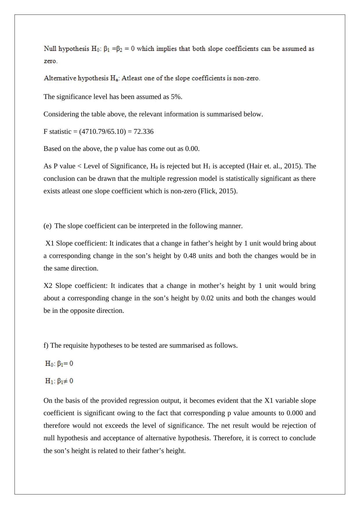
The significance level has been assumed as 5%.
Considering the table above, the relevant information is summarised below.
F statistic = (4710.79/65.10) = 72.336
Based on the above, the p value has come out as 0.00.
As P value < Level of Significance, H0 is rejected but H1 is accepted (Hair et. al., 2015). The
conclusion can be drawn that the multiple regression model is statistically significant as there
exists atleast one slope coefficient which is non-zero (Flick, 2015).
(e) The slope coefficient can be interpreted in the following manner.
X1 Slope coefficient: It indicates that a change in father’s height by 1 unit would bring about
a corresponding change in the son’s height by 0.48 units and both the changes would be in
the same direction.
X2 Slope coefficient: It indicates that a change in mother’s height by 1 unit would bring
about a corresponding change in the son’s height by 0.02 units and both the changes would
be in the opposite direction.
f) The requisite hypotheses to be tested are summarised as follows.
On the basis of the provided regression output, it becomes evident that the X1 variable slope
coefficient is significant owing to the fact that corresponding p value amounts to 0.000 and
therefore would not exceeds the level of significance. The net result would be rejection of
null hypothesis and acceptance of alternative hypothesis. Therefore, it is correct to conclude
the son’s height is related to their father’s height.

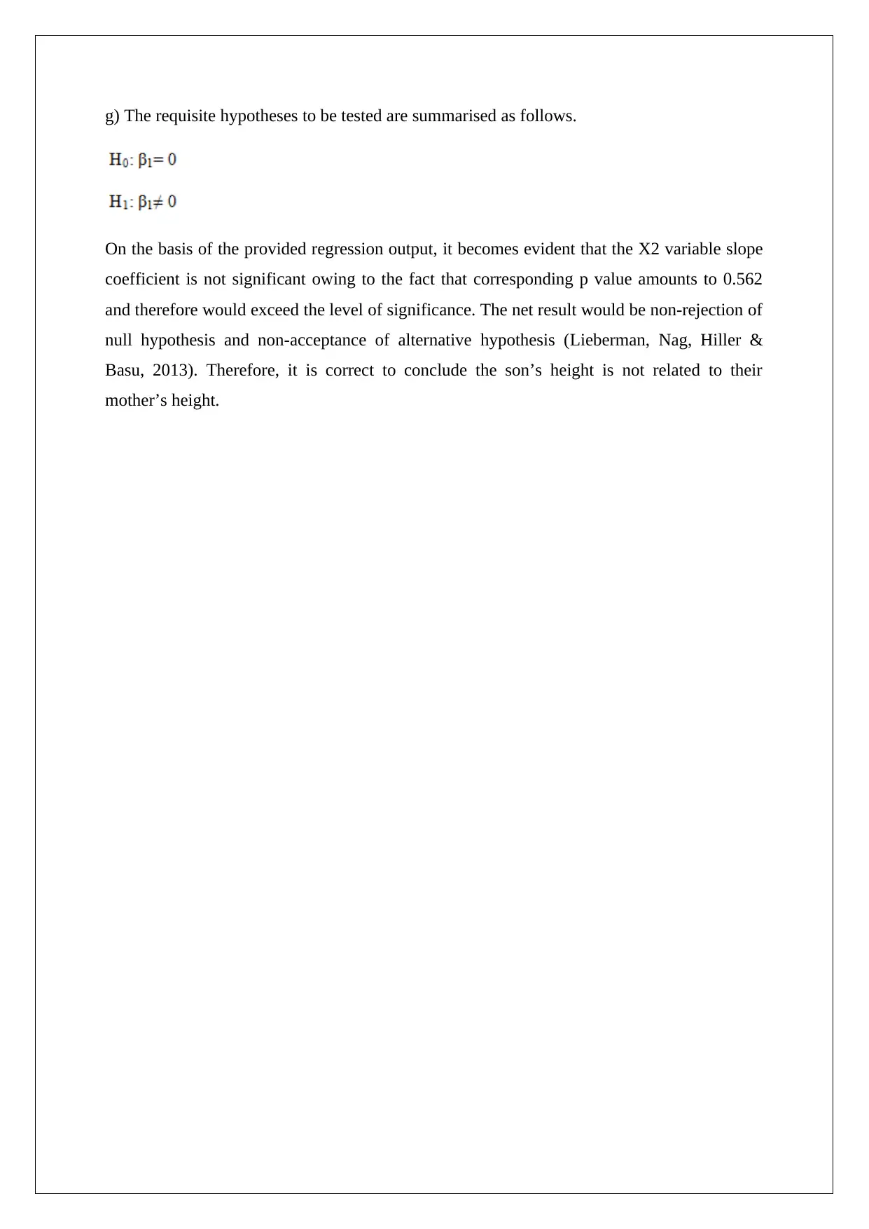
g) The requisite hypotheses to be tested are summarised as follows.
On the basis of the provided regression output, it becomes evident that the X2 variable slope
coefficient is not significant owing to the fact that corresponding p value amounts to 0.562
and therefore would exceed the level of significance. The net result would be non-rejection of
null hypothesis and non-acceptance of alternative hypothesis (Lieberman, Nag, Hiller &
Basu, 2013). Therefore, it is correct to conclude the son’s height is not related to their
mother’s height.

References
Eriksson, P. & Kovalainen, A. (2015) Quantitative methods in business research. 3rd ed.
London: Sage Publications.
Fehr, F. H. & Grossman, G. (2013). An introduction to sets, probability and hypothesis
testing. 3rd ed. Ohio: Heath.
Flick, U. (2015) Introducing research methodology: A beginner's guide to doing a research
project. 4th ed. New York: Sage Publications.
Hair, J. F., Wolfinbarger, M., Money, A. H., Samouel, P., & Page, M. J. (2015) Essentials of
business research methods. 2nd ed. New York: Routledge.
Hastie, T., Tibshirani, R. & Friedman, J. (2014) The Elements of Statistical Learning. 4th
ed. New York: Springer Publications.
Hillier, F. (2016) Introduction to Operations Research. 6th ed. New York: McGraw Hill
Publications.
Lieberman, F. J., Nag, B., Hiller, F.S. & Basu, P. (2013) Introduction To Operations
Research. 5th ed. New Delhi: Tata McGraw Hill Publishers.
Medhi, J. (2016) Statistical Methods: An Introductory Text. 4th ed. Sydney: New Age
International.