Biostatistics Assignment on Malaria Drugs and Hospitalization Cost

This assignment covers topics on biostatistics including analysis of malaria drugs and hospitalization cost. It includes qnormal plot, confidence interval, independent sample t-test, paired sample t-test and binomial distribution. The assignment is for the course HSH746/HSH946 Biostatistics 1 at a university in a city and state.

HSH746/HSH946 ASSIGNMENT 1
HSH746/HSH946 BIOSTATISTICS 1
Course
Professor’s Name
University
The City and State
Date

HSH746/HSH946 ASSIGNMENT 2
Question 1
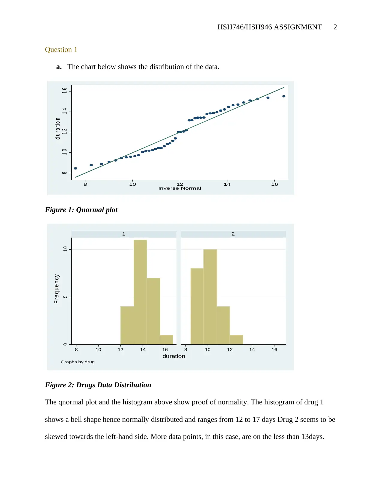
a. The chart below shows the distribution of the data.
8 1 0 1 2 1 4 1 6
d u r a t i o n
8 10 12 14 16
Inverse Normal
Figure 1: Qnormal plot
0 5 1 0
8 10 12 14 16 8 10 12 14 16
1 2
F re q u e n c y
duration
Graphs by drug
Figure 2: Drugs Data Distribution
The qnormal plot and the histogram above show proof of normality. The histogram of drug 1
shows a bell shape hence normally distributed and ranges from 12 to 17 days Drug 2 seems to be
skewed towards the left-hand side. More data points, in this case, are on the less than 13days.

HSH746/HSH946 ASSIGNMENT 3
b. Confidence Interval
A confidence interval is the range of values from which one is sure that his/her true values in the
dataset will be found.
It is given by the formula;
Confidence interval (C.I) is given by  ∓ z where -population mean, z is the z score and ()
the standard error ( σ
√ n )
Stata command qnorm duration
by drug, sort : summarize duration
histogram duration, frequency by(drug)
by drug, sort : summarize duration, detail
duration 23 10.05609 .1847525 9.672934 10.43924
Variable Obs Mean Std. Err. [95% Conf. Interval]
-> drug = 2
duration 23 13.92652 .2117428 13.48739 14.36565
Variable Obs Mean Std. Err. [95% Conf. Interval]
-> drug = 1
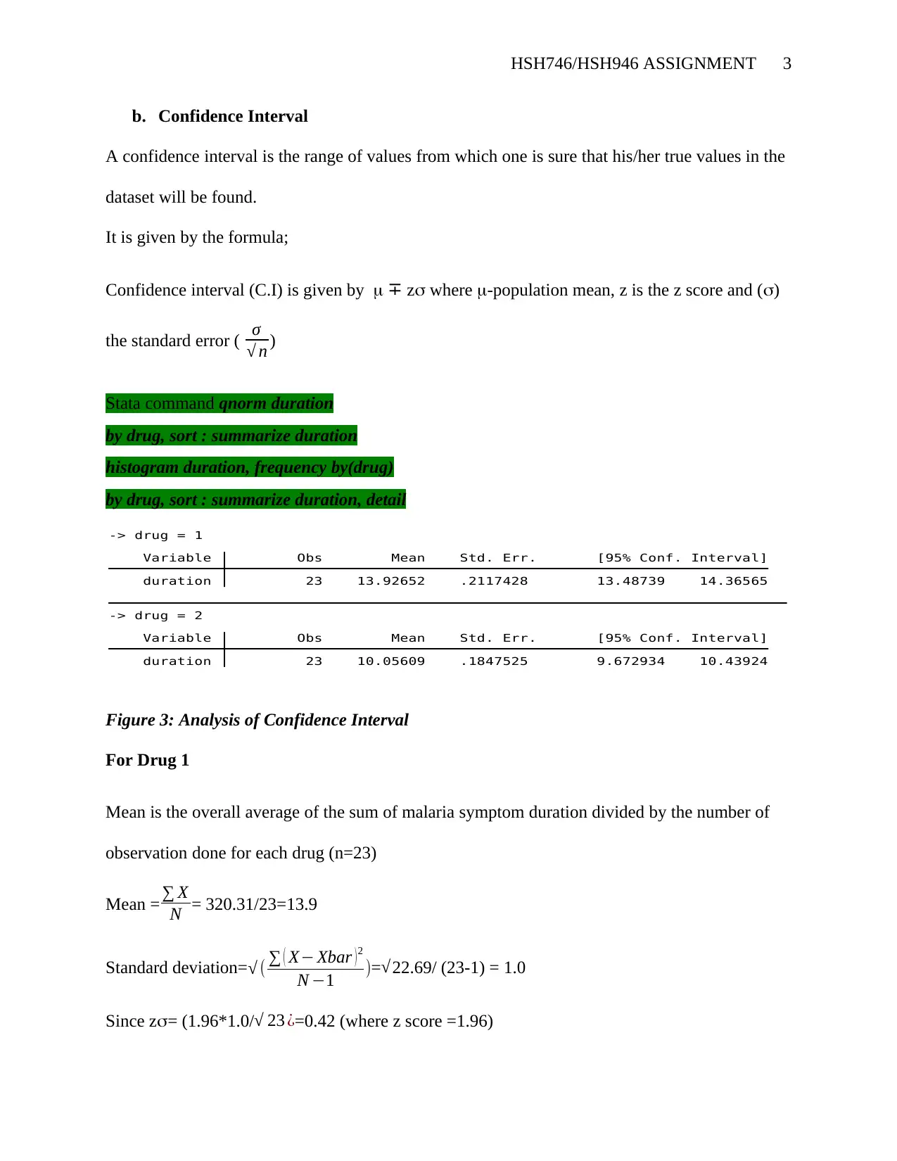
Figure 3: Analysis of Confidence Interval
For Drug 1
Mean is the overall average of the sum of malaria symptom duration divided by the number of
observation done for each drug (n=23)
Mean = ∑ X
N = 320.31/23=13.9
Standard deviation=√ ( ∑ ( X− Xbar )2
N −1 )=√22.69/ (23-1) = 1.0
Since z= (1.96*1.0/√ 23 ¿=0.42 (where z score =1.96)

HSH746/HSH946 ASSIGNMENT 4
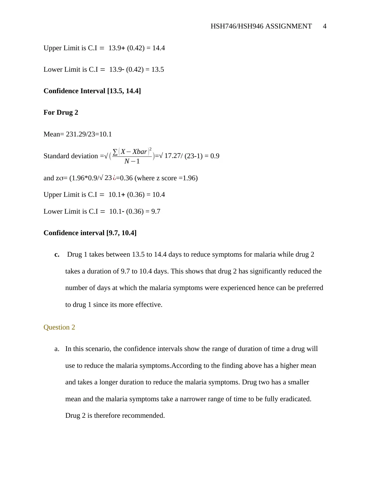
Upper Limit is C.I  13.9 (0.42) = 14.4
Lower Limit is C.I  13.9 (0.42) = 13.5
Confidence Interval [13.5, 14.4]
For Drug 2
Mean= 231.29/23=10.1
Standard deviation =√ ( ∑ ( X− Xbar )2
N −1 )=√ 17.27/ (23-1) = 0.9
and z= (1.96*0.9/√ 23 ¿=0.36 (where z score =1.96)
Upper Limit is C.I  10.1 (0.36) = 10.4
Lower Limit is C.I  10.1 (0.36) = 9.7
Confidence interval [9.7, 10.4]
c. Drug 1 takes between 13.5 to 14.4 days to reduce symptoms for malaria while drug 2
takes a duration of 9.7 to 10.4 days. This shows that drug 2 has significantly reduced the
number of days at which the malaria symptoms were experienced hence can be preferred
to drug 1 since its more effective.
Question 2
a. In this scenario, the confidence intervals show the range of duration of time a drug will
use to reduce the malaria symptoms.According to the finding above has a higher mean
and takes a longer duration to reduce the malaria symptoms. Drug two has a smaller
mean and the malaria symptoms take a narrower range of time to be fully eradicated.
Drug 2 is therefore recommended.

HSH746/HSH946 ASSIGNMENT 5
Question 3
a. An independent sample t-test can be used when the data involved is from independent
population and was obtained in a random manner where each observation had an equal
chance. Since the two drugs were obtained from independent populations, an independent
sample t-test can be carried out to compare the means of the two drugs and provide if the
two variables are significantly different
B and c
The Null Hypothesis is H0: (μ1- μ2) = 0 where μ1is the mean before and μ2 is the mean
after the intervention and the Alternative Hypothesis (H1): (μ1- μ2) >0
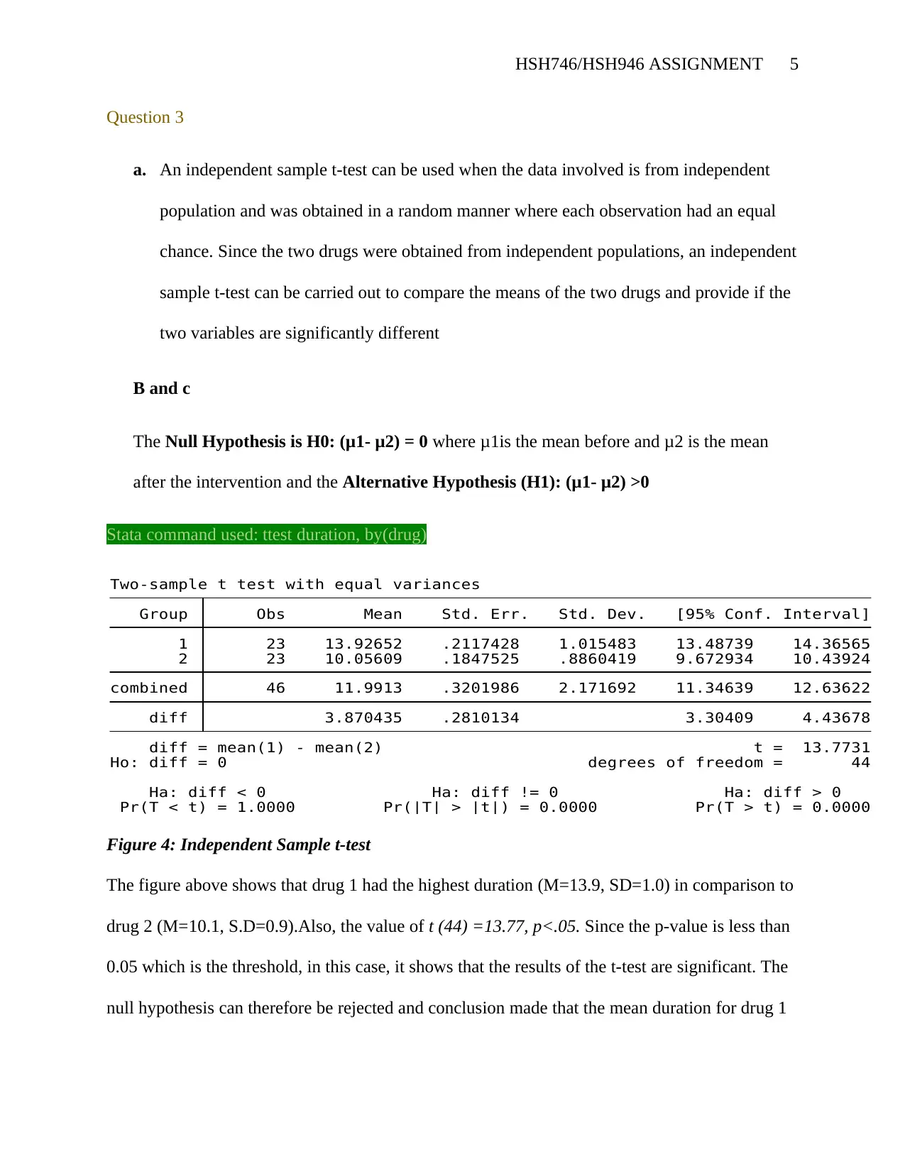
Stata command used: ttest duration, by(drug)
Pr(T < t) = 1.0000 Pr(|T| > |t|) = 0.0000 Pr(T > t) = 0.0000
Ha: diff < 0 Ha: diff != 0 Ha: diff > 0
Ho: diff = 0 degrees of freedom = 44
diff = mean(1) - mean(2) t = 13.7731
diff 3.870435 .2810134 3.30409 4.43678
combined 46 11.9913 .3201986 2.171692 11.34639 12.63622
2 23 10.05609 .1847525 .8860419 9.672934 10.43924
1 23 13.92652 .2117428 1.015483 13.48739 14.36565
Group Obs Mean Std. Err. Std. Dev. [95% Conf. Interval]
Two-sample t test with equal variances
Figure 4: Independent Sample t-test
The figure above shows that drug 1 had the highest duration (M=13.9, SD=1.0) in comparison to
drug 2 (M=10.1, S.D=0.9).Also, the value of t (44) =13.77, p<.05. Since the p-value is less than
0.05 which is the threshold, in this case, it shows that the results of the t-test are significant. The
null hypothesis can therefore be rejected and conclusion made that the mean duration for drug 1

HSH746/HSH946 ASSIGNMENT 6
is different from drug 2.This means duration that the mean duration for drug 2 is slightly smaller
than drug 1.
Question 4
a. This question utilizes the paired sample t-test knowledge. This is where an experiment is
measured before and after an intervention. In this case, the hospitalization cost of patients
was measured before and after an intervention.This test, therefore, calculates and
compares the means of the hospitalization costs at these two intervals and tries to match
if there exist statistically significant difference.
The Null Hypothesis is H0: (μ1- μ2) = 0 where μ1is the mean before and μ2 is the mean after
the intervention and the Alternative Hypothesis (H1): (μ1- μ2) ≠ 0
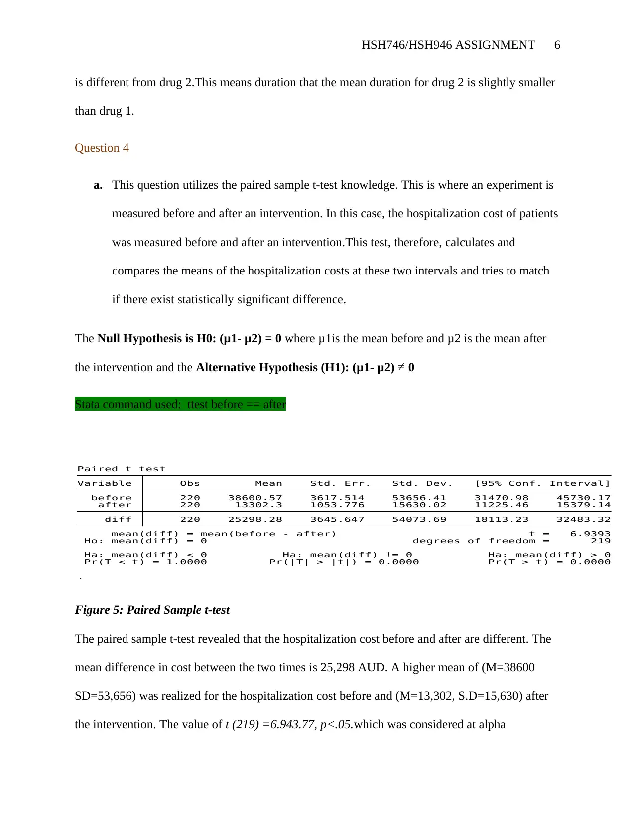
Stata command used: ttest before == after
.
Pr(T < t) = 1.0000 Pr(|T| > |t|) = 0.0000 Pr(T > t) = 0.0000
Ha: mean(diff) < 0 Ha: mean(diff) != 0 Ha: mean(diff) > 0
Ho: mean(diff) = 0 degrees of freedom = 219
mean(diff) = mean(before - after) t = 6.9393
diff 220 25298.28 3645.647 54073.69 18113.23 32483.32
after 220 13302.3 1053.776 15630.02 11225.46 15379.14
before 220 38600.57 3617.514 53656.41 31470.98 45730.17
Variable Obs Mean Std. Err. Std. Dev. [95% Conf. Interval]
Paired t test
Figure 5: Paired Sample t-test
The paired sample t-test revealed that the hospitalization cost before and after are different. The
mean difference in cost between the two times is 25,298 AUD. A higher mean of (M=38600
SD=53,656) was realized for the hospitalization cost before and (M=13,302, S.D=15,630) after
the intervention. The value of t (219) =6.943.77, p<.05.which was considered at alpha

HSH746/HSH946 ASSIGNMENT 7
=0.05.This suggests that there exist a statically significant difference in hospitalization cost
before and after the intervention.
b. There is, therefore, enough statistical evidence that that the new intervention has resulted
in a huge decrease in the hospitalization cost hence should be adopted to save resources.
Rejecting the null hypothesis implies that the mean differences between the two cost are
not equal to 0
Question 5
The distribution represented here is a binomial distribution. This is where there is a probability of
success or failure in an experiment.
The population proportion is the fraction of the total number of successful events that
were registered in an event divided by the total occurrences.i.e proportion (p hat) = m / n
Considering that m is the number of successes achieved and n is the sample size
a. The total number of children that received vaccination are 513 while they that did not are
487. Proportion=513/1000= 0.513= 0.51 (2.dp)
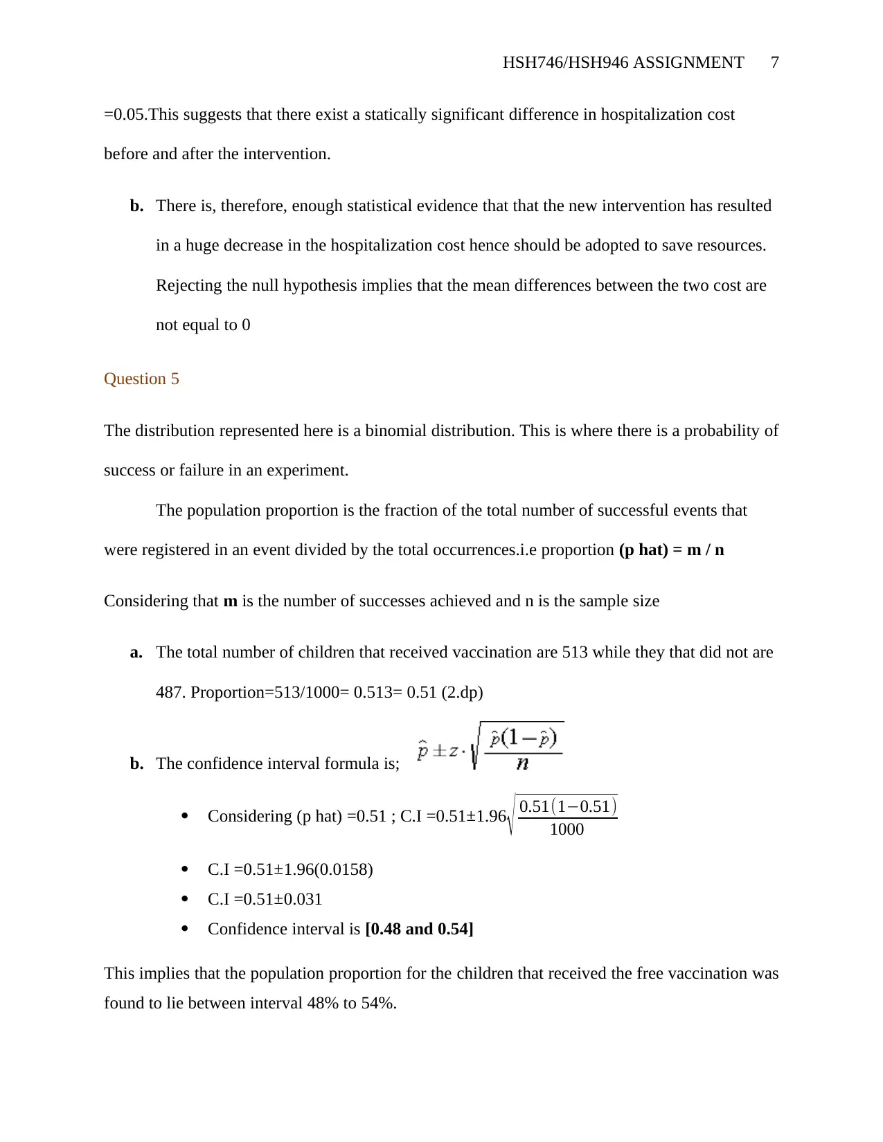
b. The confidence interval formula is;
 Considering (p hat) =0.51 ; C.I =0.51±1.96
√ 0.51(1−0.51)
1000
 C.I =0.51 ±1.96(0.0158)
 C.I =0.51 ±0.031
 Confidence interval is [0.48 and 0.54]
This implies that the population proportion for the children that received the free vaccination was
found to lie between interval 48% to 54%.

HSH746/HSH946 ASSIGNMENT 8