Data Mining Business Case Analysis: PCA, Naive Bayes, and Strategy

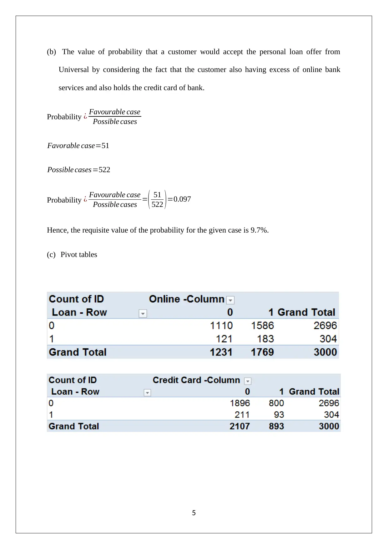
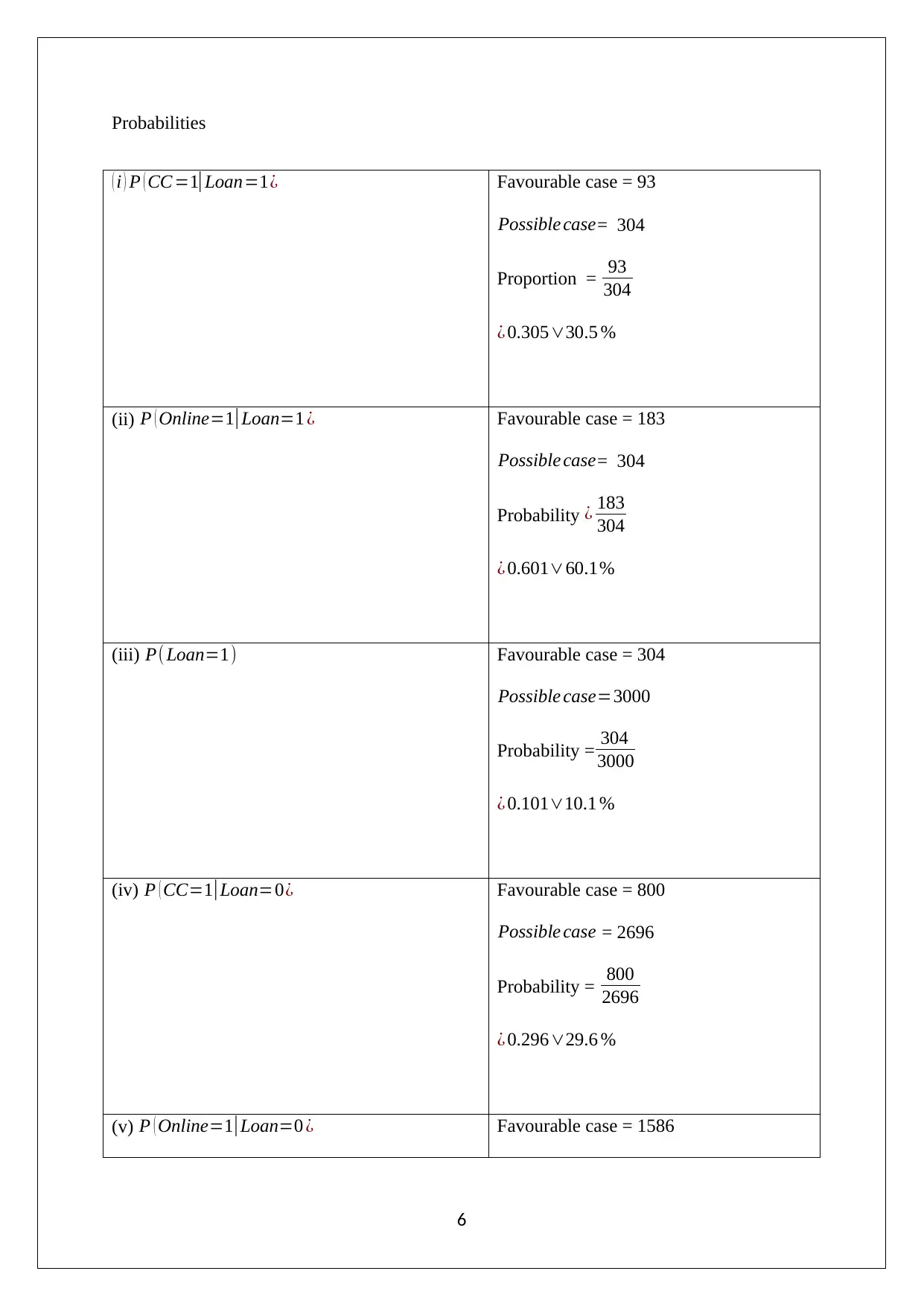
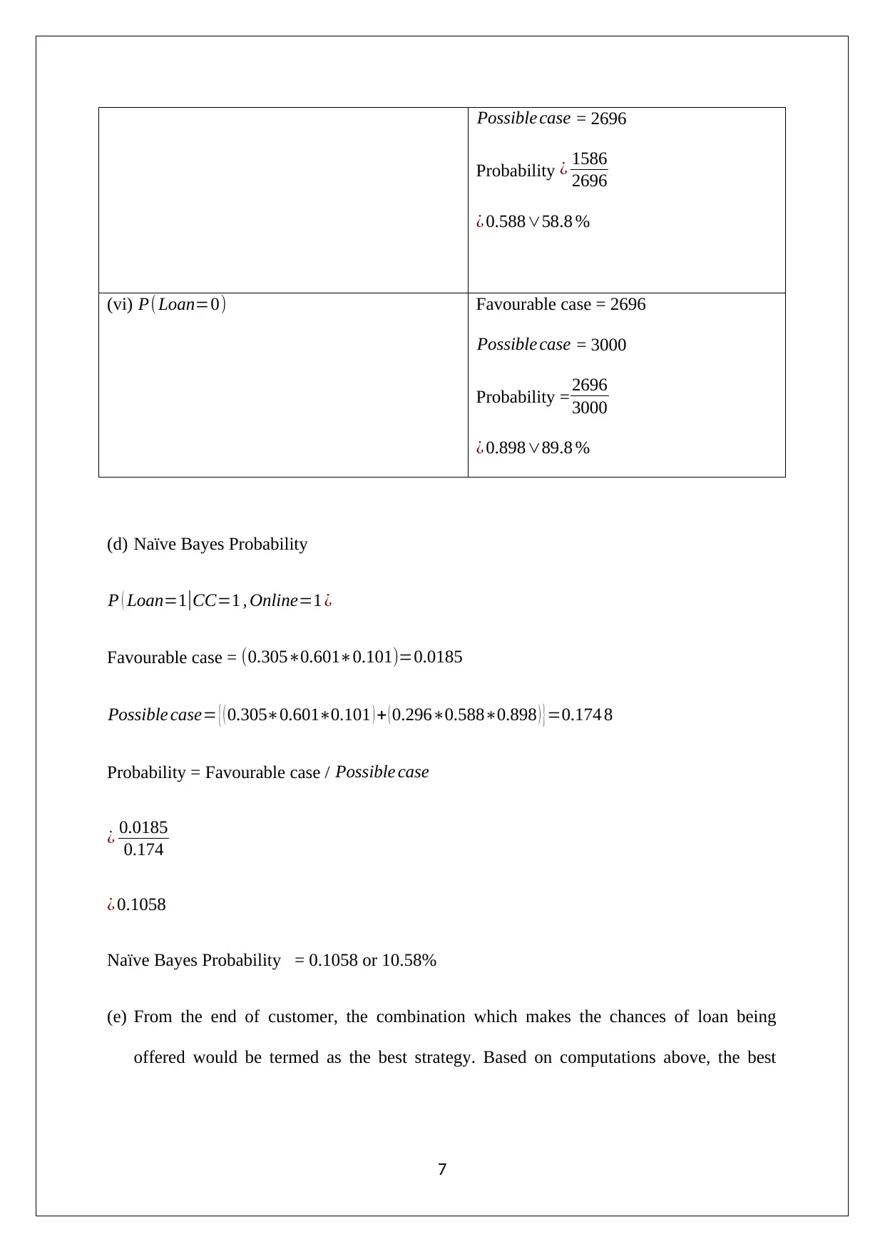
This assignment presents a data mining business case analysis, focusing on Principal Component Analysis (PCA) and Naive Bayes techniques. The analysis begins with an examination of PCA, including the identification of significant principal components and their relation to firm performance, financial returns, operational efficiency, and variable electricity costs. It addresses normalization issues and outlines the advantages and limitations of PCA. The second part of the assignment utilizes the XLMiner tool to generate training data and explores customer behavior in relation to loan acceptance, online banking services, and credit card usage. Pivot tables and Naive Bayes probability calculations are used to determine the best customer strategy to increase the probability of loan acceptance. The analysis concludes with the identification of the optimal customer strategy based on the computed probabilities.

DATA MINING
BUSINESS CASE ANALYSIS
[Pick the date]
STUDENT ID

Question 1
a) One of the key results of the PCA is the component matrix which represents the Eigen
values related to each particular feature. The respective scores can be derived from the
equation derived through the use of this matrix. Further, the respective significance of the
principal components is reflected from the extent of total variance that it accounts for,
which is on account of the higher importance being provided to components that lead to
higher variance. Further, the principal components which have very limited contribution to
the total variance are not considered significant and are ignored. The relevant output of
PCA analysis as obtained from XLMiner is reflected below.
The first step is to identify the number of principal components that should be considered.
Assuming that only 80% of the variance needs to be explained, the PCA matrix can shift
focus to only the first four principal components while ignoring the rest. In order to
understand which aspect is being captured by these principal components in relation to the
1

firm’s performance, it is imperative to identify the features that the significant principal
components focus on. This is apparent from the following analysis.
 With regards to the first principal component, the essential parameters based on
highest values are x1(income to debt) and x2(rate of return). Hence, this component is
representative of the financial returns.
 With regards to the second principal component, the essential parameters based on
highest values are x4(Annual Load Factor) and x8(Total fuel costs). Hence, this
component is representative of the operational efficiency.
 With regards to the third principal component, the essential parameters based on
highest values are x3(Cost per unit) and x7(Percent nuclear). Hence, this component
is representative of the variable electricity cost.
 With regards to the fourth principal component, the essential parameters based on
highest values are x1(income to debt) and x3(Cost per unit). Hence, this component is
representative of the financial performance.
Normalisation
One of the potential issues with PCA can be in the form of distorting effect of the scales of
the given variables. Owing to this, it may so happen that a particular variable tends to
undermine the importance of the others by ensuring that the first principal component
accounts for a very high contribution to total variance. This is not the importance of the
variance but rather the large range of scale. In such cases, normalisation is done to convert
variables into normal form and hence ensure that the principal components significance can
be correctly established. It is not required here on account of the total variance matrix where
no domination of a single variable occurs.
(b) The central advantages and limitations of principal component analysis is outlined below:
2

Central Advantages
Reduction of complex data set into simpler data sets
Determination the actual structure of the data set
Reduction of the multi-dimensional variables into fewer dimensional variables
Easy to evaluate the result because the principal components are distributed in the
orthogonal format
Visualization of principal component vector is easy because the cloud points are arranged
into either in m- dimensional space or p-dimensional space.
Even if the variables are reduced in PCA, but the principal components are representing
the original data only.
Central Limitations
It is valid only for those data variables which demonstrate predominantly linear relations.
It cannot apply when the data set has been taken from blind source data.
The direction of max-variance principal components is difficult to determine because the
principal components are distributed in the multi-dimensional space in which each of the
principal component has its own axis and also, each of the axis are exactly at the right
angle side of the another principal component.
The given data which cannot be captured by mean and variance would not be analysed
with the help of PCA techniques and hence, the other imperative method such as
Independent Component Analysis would be used.
It cannot be applied when the variable data belongs to the categorical type.
Question 2
3

(a) In order to generate the training data from course data of 5000, XLMiner tool was used
for data mining and visualization has been taken into consideration.
60% training and 40% validation would be used in the standard partition in XLMiner.
The training data comprises 3000 data set with 14 different variables such as age, online,
loan, credit card and so on. The two predictors are Online and Credit Card.
Pivot table
Credit card
CC = 0 “Customer of Universal Bank does not own the credit card”
CC = 1 “Customer of Universal Bank owns the credit card”
Loan
Loan = 0 “Customer of Universal Bank does not accept the personal loan offer”
Loan = 1 “Customer of Universal Bank accepts the personal loan offer”
Online
Online = 0 “Customer of Universal Bank does not use the online net banking service”
Online = 1 “Customer of Universal Bank usages the online net banking service”
4

(b) The value of probability that a customer would accept the personal loan offer from
Universal by considering the fact that the customer also having excess of online bank
services and also holds the credit card of bank.
Probability ¿ Favourable case
Possible cases
Favorable case=51
Possible cases =522
Probability ¿ Favourable case
Possible cases =( 51
522 )=0.097
Hence, the requisite value of the probability for the given case is 9.7%.
(c) Pivot tables
5

Probabilities
( i ) P ( CC =1|Loan=1¿ Favourable case = 93
Possible case= 304
Proportion = 93
304
¿ 0.305∨30.5 %
(ii) P ( Online=1|Loan=1 ¿ Favourable case = 183
Possible case= 304
Probability ¿ 183
304
¿ 0.601∨60.1%
(iii) P( Loan=1) Favourable case = 304
Possible case=3000
Probability = 304
3000
¿ 0.101∨10.1 %
(iv) P ( CC=1|Loan=0¿ Favourable case = 800
Possible case = 2696
Probability = 800
2696
¿ 0.296∨29.6 %
(v) P ( Online=1|Loan=0 ¿ Favourable case = 1586
6

Possible case = 2696
Probability ¿ 1586
2696
¿ 0.588∨58.8 %
(vi) P(Loan=0) Favourable case = 2696
Possible case = 3000
Probability = 2696
3000
¿ 0.898∨89.8 %
(d) Naïve Bayes Probability
P ( Loan=1|CC=1 , Online=1 ¿
Favourable case = (0.305∗0.601∗0.101)=0.0185
Possible case= { ( 0.305∗0.601∗0.101 ) + ( 0.296∗0.588∗0.898 ) }=0.174 8
Probability = Favourable case / Possible case
¿ 0.0185
0.174
¿ 0.1058
Naïve Bayes Probability = 0.1058 or 10.58%
(e) From the end of customer, the combination which makes the chances of loan being
offered would be termed as the best strategy. Based on computations above, the best
7