Data Mining on Twitter Data using Machine Learning Algorithms

This is as a result of the number of individual that gets to tweet misleading tweets is lower as compared to the number of individual that tweet relevant tweets(Arora et al., 2018). This is as a result of the number of individual that gets to tweet misleading tweets is lower as compared to the number of individual that tweet relevant tweets(Arora et al., 2018).

Data mining on twitter data using machine learning algorithms in R
Executive summary
Twitter is and has been popular since its development and launch into internet system over the
years. The popularity of twitter over the years has attracted large number of subscribers hence
brought on board various groups of people that tweet on tweeter platforms. This has resulted
from several evidence of experiencing spam tweets, long sides’ reliable tweets that were tweeted
on the forum.
Occurrence of Advertisement in tweeter is as a result of tweets that are transmitted yet they have
the wrong information to the consumers. Most social communication and mail platforms try as
much as possible to limit having misleading advertisement and mails. This has led to most of the
forums to develop clear system on how to categorize emails as misleading or not misleading.
This has resulted to screening of misleading mails and contents in most occurrences by the
developed systems and after the assessment, the system decides whether the content is
misleading or not. In instance where the content is found to have been misleading the consumers,
decisions will be made depending on the forum and its influence left out to the consumers or it
may be erased from the system or moved to the misleading section of the system. This study
therefore brings about the use of train and test datasets to group twitter data sets. The response
variable has two groups of different character, the first group is the spammers (misleading
adverts) and the other is the non-spammers. Tweet -class is the response variable, which will be
referred to when elaborating R-programming .This programming is used in development of five
machine learning categories including algorithms.
Key words –Data set, Twitter, algorithms, R

Introduction
Machine learning is important in daily operation of companies that have adopted its use.
Machine learning has been adopted from manufacturing to Agriculture companies to sales and
finally to health care system .Machine learning and artificial intelligence has impacted on lives
and increased the profit margins .Machine learning can be largely used in categorizing and
regression, and all that involves future predictions (Cordon Et al., 2018).Cases arising from
misleading tweets will be addressed by use of categorizes in R-analytics software.
Train dataset, test dataset one and two have been provided for classification. Theoretically and
practically, it is obvious to find a number of misleading tweet . Total is always slower than the
accurate information, hence leading to unknown data that is passed through the trained model to
give the same scenario. This is as a result of the number of individual that gets to tweet
misleading tweets is lower as compared to the number of individual that tweet relevant
tweets(Kumari,Vidya $Karitha,2019).The number of models that are to developed is five. From
the list of the classification models, some were unsupervised while others were supervised. Of
the list of the supervised learning, we get to have; decision trees, random forest, logistics
regression and naïve Bayes. The only unsupervised algorithm that will be applied is the; K-
means clustering (Arora et al., 2018).
Literature review
The machine learning process will be dependent on classification ,this will be translated into
clusters .Classified data are the only groups to be clustered. In supervised learning, a system is
instructed on what to do after being trained while in unsupervised learning, the reverse occurs .
Unsupervised learning connects the dots on its own from the fed data and makes a judgment of

its own from the data, hence ease in categorization as one develops a reliable model and let it
to run hence future predictions with the help of a constant amount of data to be tested. The only
time one needs to change the bits of the developed model is when a new data set of train is
provided. In models developments, there is a need to have a train and a test data set. These can
be obtained from the main data set that is provided in a model by actually splitting into two to
give both train and test data sets (Bowers, Alex & Xiaoliang Zhou, 2019).
Of the performance metrics, there will be need to use confusion matrix, ROC and the AUC
curves to sort out the test of a performance problem. The remaining two performance matrices
are by checking the actual percentage performance of the test data 1 against test data 2 and the
actual error rates that the tested data sets do provide when running over respective developed
models (Bowers, Alex and Xiaoliang Zhou, 2019).
Supervised and unsupervised machine learning algorithms and their importance
The first choice of classification is the logistic regression ,which is a statistical model that uses
the binomial outcome to determine the classification, the relationship of a response variable
based on other predictor variables identified. In the process, probabilities are established.
Logistic regression is more of a classification ,algorithm in R as it is a predictive algorithm and
the reason is if predictive variable happens then response variable is classified as either one or
the other and this can be run on test data. Once test data has been used for prediction using the
already developed model, the performance model itself can be tested by using a confusion
matrix, ROC curve and AUC (Gelman et al. 2019).
The next classification model is the decision tree. This classification model uses nodes to get to
branches which then divide into further branches and later into more branches hence giving a
classification leaves of the response variable in question. The performance of this model is tested

by the use of cross-validation plot. If the plot is not well promising then printing can be made on
the tree to have a clearer classifications. The pruning and predicting is the test performance
matrix (Chen et al. 2018).
The third model will be the naïve Bayes and the evaluation matrix will be the plot of the actual
models together with the confusion matrix that is gotten from the results of the model when
running (slamet et al. 2018)
The fourth model to be considered will be the Random forest and in this case, classification will
be done by the use of several artificial trees in the random forest that can be gotten by the use of
the random forest library that is there in R. The evaluation matrix will be the confusion matrix
add the rf plot that helps sees the actual error rate and where actually the model cannot be
improved further and at what number of trees in total is considered in the classification process
(Subudhi et al. 2019).
Development of classification algorithms
The datasets provided, were in form of text files , were loaded and viewed in R .The dataset is a
data frame that is in a single column each. Only when doing text mining or Natural language
processing one gets to use such datasets. For our case, the data frames must be converted into a
CSV file from the text files. After conversion, the variable or attribute names are given as per
the JSON format provided in the listing of how the dataset should be.
From here we will be diving deep into the classification model. We will be focusing on logistic
regression , first of all, upload all the data sets. We have train data and two test data sets. The
models will be developed using the provided train data and then tested using the provided test
datasets. All the test data sets must be used to make predictions , the reason is that the
performance of both the datasets need to be compared to help rule out which test data is the best

for use and which is not. All the steps will be illustrated and the results will be explained as well
as how every model is being explored to completion and perfection. This is to help bring about
stepwise understanding.
Technical demostration
Starting with the logistic regression model, all the three CSV converted datasets will be loaded
on to an R script and then cleaning will be done . The exhibit 1 below shows the loading of the
train data and loading of tools package that aid in the manipulation of data sets;
exhibit 1.
The clean up of the data , in this case, there was fill-up of the missing data entries that were there
in the second data frame,hence it is to be corrected by the use of the ‘mice' and the VIM libraries
(Thioulouse et al. 2018).

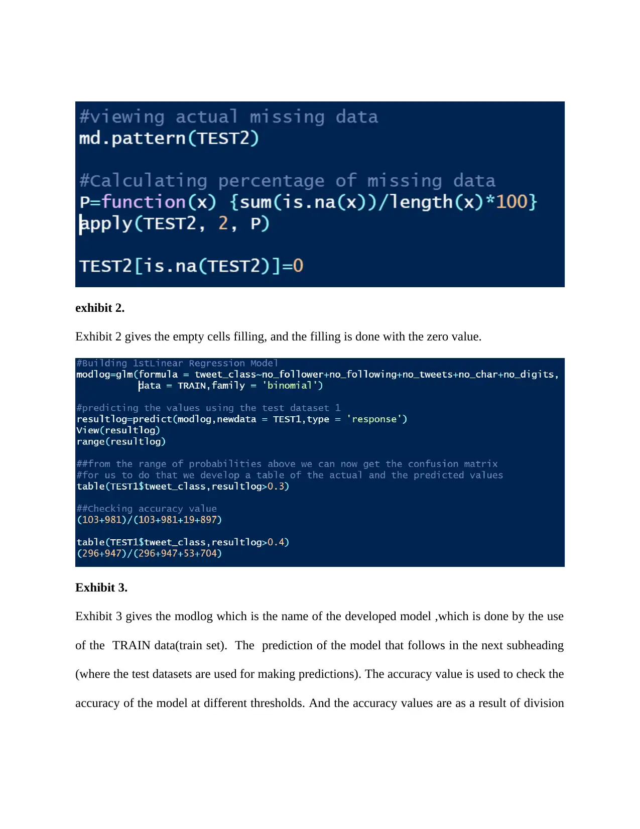
exhibit 2.
Exhibit 2 gives the empty cells filling, and the filling is done with the zero value.
Exhibit 3.
Exhibit 3 gives the modlog which is the name of the developed model ,which is done by the use
of the TRAIN data(train set). The prediction of the model that follows in the next subheading
(where the test datasets are used for making predictions). The accuracy value is used to check the
accuracy of the model at different thresholds. And the accuracy values are as a result of division

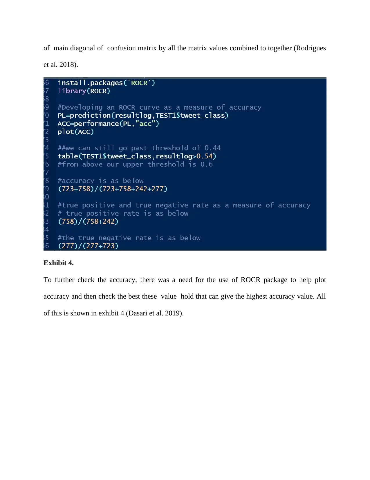
of main diagonal of confusion matrix by all the matrix values combined to together (Rodrigues
et al. 2018).
Exhibit 4.
To further check the accuracy, there was a need for the use of ROCR package to help plot
accuracy and then check the best these value hold that can give the highest accuracy value. All
of this is shown in exhibit 4 (Dasari et al. 2019).

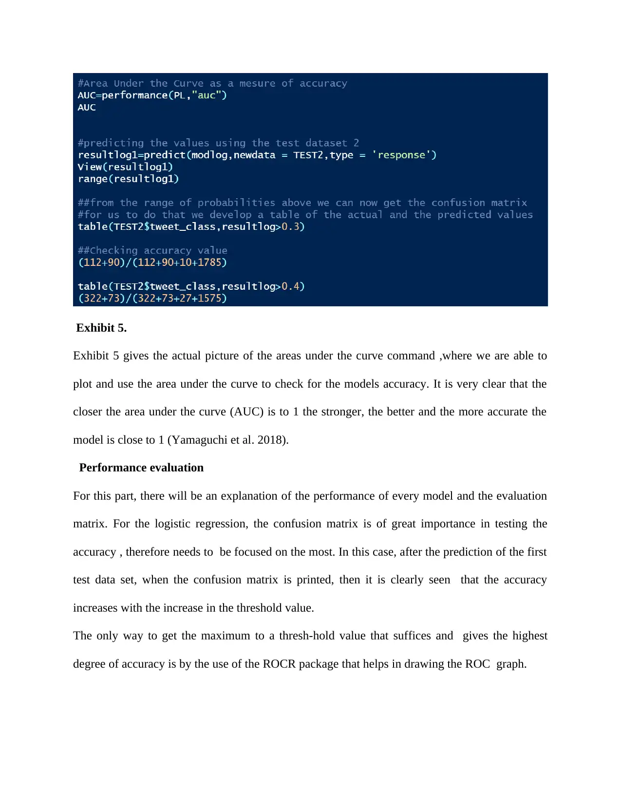
Exhibit 5.
Exhibit 5 gives the actual picture of the areas under the curve command ,where we are able to
plot and use the area under the curve to check for the models accuracy. It is very clear that the
closer the area under the curve (AUC) is to 1 the stronger, the better and the more accurate the
model is close to 1 (Yamaguchi et al. 2018).
Performance evaluation
For this part, there will be an explanation of the performance of every model and the evaluation
matrix. For the logistic regression, the confusion matrix is of great importance in testing the
accuracy , therefore needs to be focused on the most. In this case, after the prediction of the first
test data set, when the confusion matrix is printed, then it is clearly seen that the accuracy
increases with the increase in the threshold value.
The only way to get the maximum to a thresh-hold value that suffices and gives the highest
degree of accuracy is by the use of the ROCR package that helps in drawing the ROC graph.

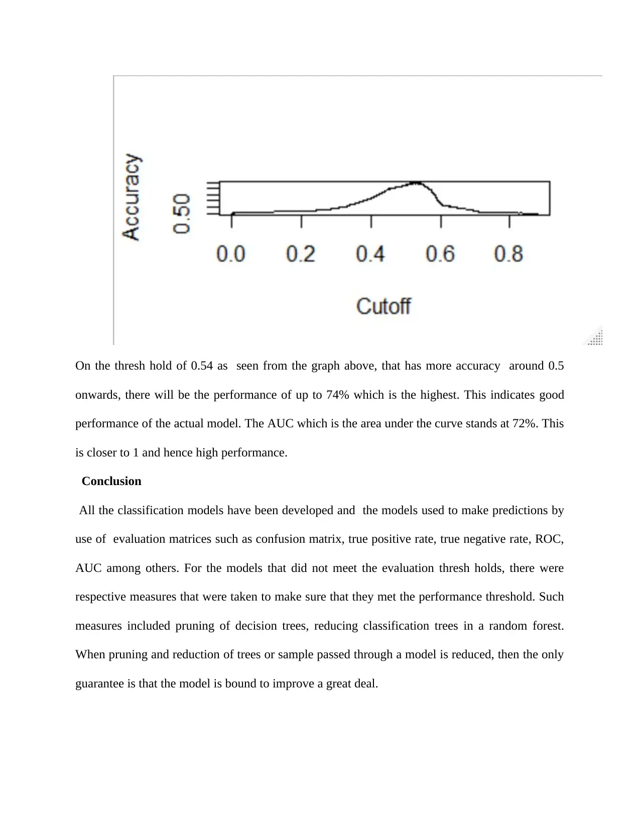
On the thresh hold of 0.54 as seen from the graph above, that has more accuracy around 0.5
onwards, there will be the performance of up to 74% which is the highest. This indicates good
performance of the actual model. The AUC which is the area under the curve stands at 72%. This
is closer to 1 and hence high performance.
Conclusion
All the classification models have been developed and the models used to make predictions by
use of evaluation matrices such as confusion matrix, true positive rate, true negative rate, ROC,
AUC among others. For the models that did not meet the evaluation thresh holds, there were
respective measures that were taken to make sure that they met the performance threshold. Such
measures included pruning of decision trees, reducing classification trees in a random forest.
When pruning and reduction of trees or sample passed through a model is reduced, then the only
guarantee is that the model is bound to improve a great deal.

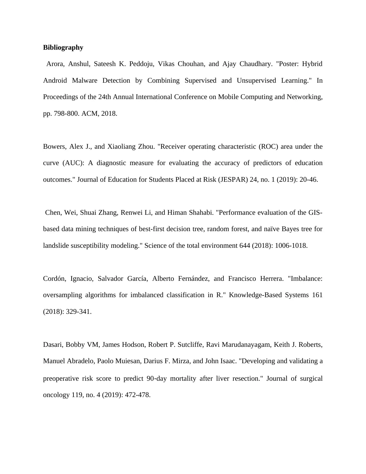
Bibliography
Arora, Anshul, Sateesh K. Peddoju, Vikas Chouhan, and Ajay Chaudhary. "Poster: Hybrid
Android Malware Detection by Combining Supervised and Unsupervised Learning." In
Proceedings of the 24th Annual International Conference on Mobile Computing and Networking,
pp. 798-800. ACM, 2018.
Bowers, Alex J., and Xiaoliang Zhou. "Receiver operating characteristic (ROC) area under the
curve (AUC): A diagnostic measure for evaluating the accuracy of predictors of education
outcomes." Journal of Education for Students Placed at Risk (JESPAR) 24, no. 1 (2019): 20-46.
Chen, Wei, Shuai Zhang, Renwei Li, and Himan Shahabi. "Performance evaluation of the GIS-
based data mining techniques of best-first decision tree, random forest, and naïve Bayes tree for
landslide susceptibility modeling." Science of the total environment 644 (2018): 1006-1018.
Cordón, Ignacio, Salvador García, Alberto Fernández, and Francisco Herrera. "Imbalance:
oversampling algorithms for imbalanced classification in R." Knowledge-Based Systems 161
(2018): 329-341.
Dasari, Bobby VM, James Hodson, Robert P. Sutcliffe, Ravi Marudanayagam, Keith J. Roberts,
Manuel Abradelo, Paolo Muiesan, Darius F. Mirza, and John Isaac. "Developing and validating a
preoperative risk score to predict 90‐day mortality after liver resection." Journal of surgical
oncology 119, no. 4 (2019): 472-478.

Gelman, Andrew, Ben Goodrich, Jonah Gabry, and Aki Vehtari. "R-squared for Bayesian
regression models." The American Statistician (2019): 1-7.
Kumari, KR Vidya, and C. R. Kavitha. "Spam Detection Using Machine Learning in R." In
International Conference on Computer Networks and Communication Technologies, pp. 55-64.
Springer, Singapore, 2019.
Rodrigues, Mark A., Neshika Samarasekera, Christine Lerpiniere, Catherine Humphreys, Mark
O. McCarron, Philip M. White, James AR Nicoll et al. "The Edinburgh CT and genetic
diagnostic criteria for lobar intracerebral haemorrhage associated with cerebral amyloid
angiopathy: model development and diagnostic test accuracy study." The Lancet Neurology 17,
no. 3 (2018): 232-240.
Slamet, Cepy, Rian Andrian, Dian Sa'adillah Maylawati, W. Darmalaksana, and M. A.
Ramdhani. "Web scraping and Naïve Bayes classification for job search engine." In IOP
Conference Series: Materials Science and Engineering, vol. 288, no. 1, p. 012038. IOP
Publishing, 2018.
Subudhi, Asit, Manasa Dash, and Sukanta Sabut. "Automated segmentation and classification of
brain stroke using expectation-maximization and random forest classifier." Biocybernetics and
Biomedical Engineering (2019).

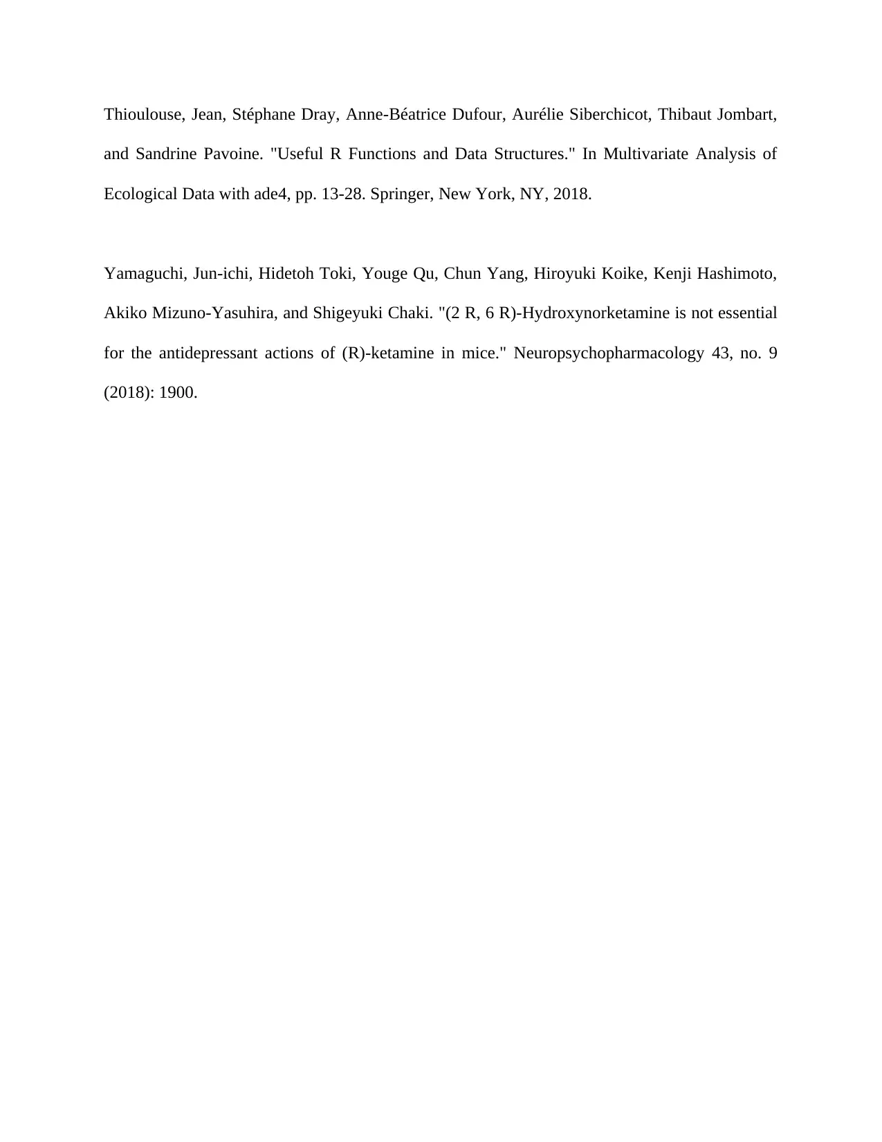
Thioulouse, Jean, Stéphane Dray, Anne-Béatrice Dufour, Aurélie Siberchicot, Thibaut Jombart,
and Sandrine Pavoine. "Useful R Functions and Data Structures." In Multivariate Analysis of
Ecological Data with ade4, pp. 13-28. Springer, New York, NY, 2018.
Yamaguchi, Jun-ichi, Hidetoh Toki, Youge Qu, Chun Yang, Hiroyuki Koike, Kenji Hashimoto,
Akiko Mizuno-Yasuhira, and Shigeyuki Chaki. "(2 R, 6 R)-Hydroxynorketamine is not essential
for the antidepressant actions of (R)-ketamine in mice." Neuropsychopharmacology 43, no. 9
(2018): 1900.