Managerial Economics Case Study

This case study analyzes the production costs and profit estimation for Harding Silicon Enterprises (HSE) in the field of RAM chip production. It includes a statistical analysis of cost functions, regression models for average variable cost (AVC) and total variable cost (TVC), and estimation of profit based on different chip prices. The study also discusses the price at which the company should shut down operations.

MANAGERIAL ECONOMICS
CASE STUDY
[DATE]
STUDENT NAME
STUDENT ID:

INTRODUCTION
The given case pertains to Harding Silicon Enterprises (HSE) which is in the business of
producing RAM chips for electronic devices. The company has provided data related to cost
and output for the past 19 months. The various cost are divided into seven categories with
some costs being fixed while the other variable. The objective of this report is to carry out a
statistical analysis of the short term production costs so as to estimate different cost functions
such as AVC (Average Variable Cost) and TVC (Total Variable Cost). For the chip prices in
two different scenarios, the production level also has been estimated along with the
forecasted profit. Finally the price in the short run which would result in shut down of
operations also has been computed.
ANALYSIS
Question 1
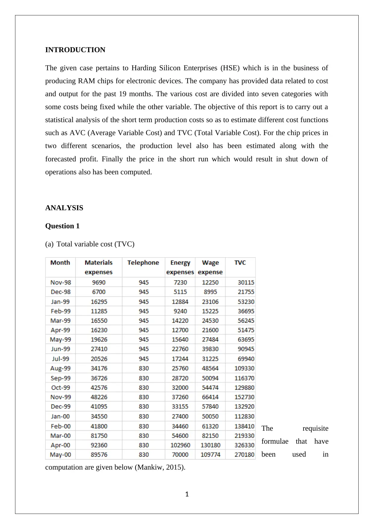
(a) Total variable cost (TVC)
The requisite
formulae that have
been used in
computation are given below (Mankiw, 2015).
1

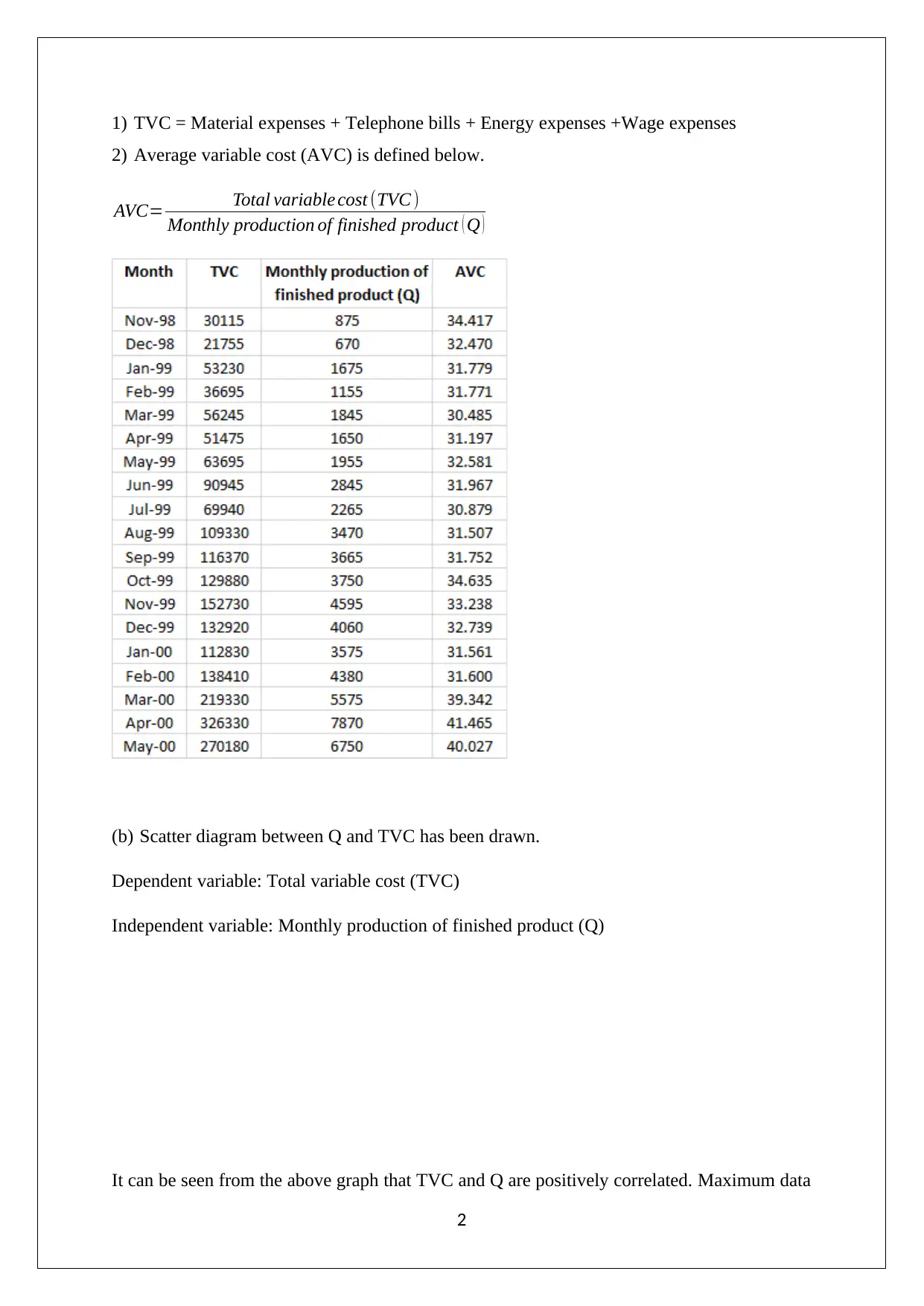
1) TVC = Material expenses + Telephone bills + Energy expenses +Wage expenses
2) Average variable cost (AVC) is defined below.
AVC= Total variable cost (TVC )
Monthly production of finished product ( Q )
(b) Scatter diagram between Q and TVC has been drawn.
Dependent variable: Total variable cost (TVC)
Independent variable: Monthly production of finished product (Q)
It can be seen from the above graph that TVC and Q are positively correlated. Maximum data
2

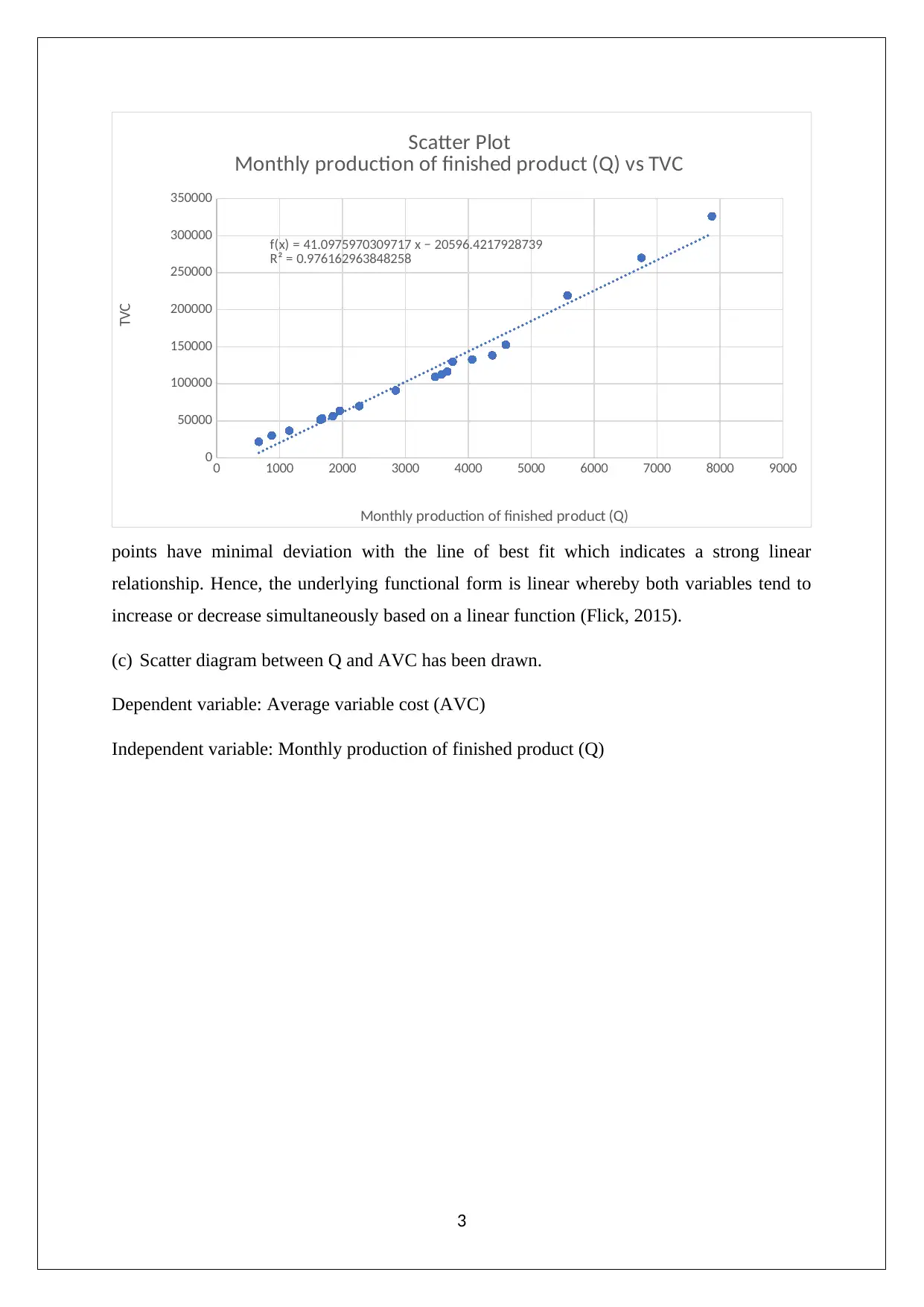
points have minimal deviation with the line of best fit which indicates a strong linear
relationship. Hence, the underlying functional form is linear whereby both variables tend to
increase or decrease simultaneously based on a linear function (Flick, 2015).
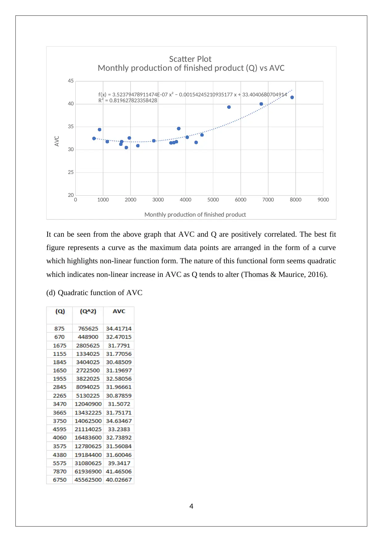
(c) Scatter diagram between Q and AVC has been drawn.
Dependent variable: Average variable cost (AVC)
Independent variable: Monthly production of finished product (Q)
3
0 1000 2000 3000 4000 5000 6000 7000 8000 9000
0
50000
100000
150000
200000
250000
300000
350000
f(x) = 41.0975970309717 x − 20596.4217928739
R² = 0.976162963848258
Scatter Plot
Monthly production of finished product (Q) vs TVC
Monthly production of finished product (Q)
TVC

0 1000 2000 3000 4000 5000 6000 7000 8000 9000
20
25
30
35
40
45
f(x) = 3.52379478911474E-07 x² − 0.00154245210935177 x + 33.4040680704914
R² = 0.819627823358428
Scatter Plot
Monthly production of finished product (Q) vs AVC
Monthly production of finished product
AVC
It can be seen from the above graph that AVC and Q are positively correlated. The best fit
figure represents a curve as the maximum data points are arranged in the form of a curve
which highlights non-linear function form. The nature of this functional form seems quadratic
which indicates non-linear increase in AVC as Q tends to alter (Thomas & Maurice, 2016).
(d) Quadratic function of AVC
4

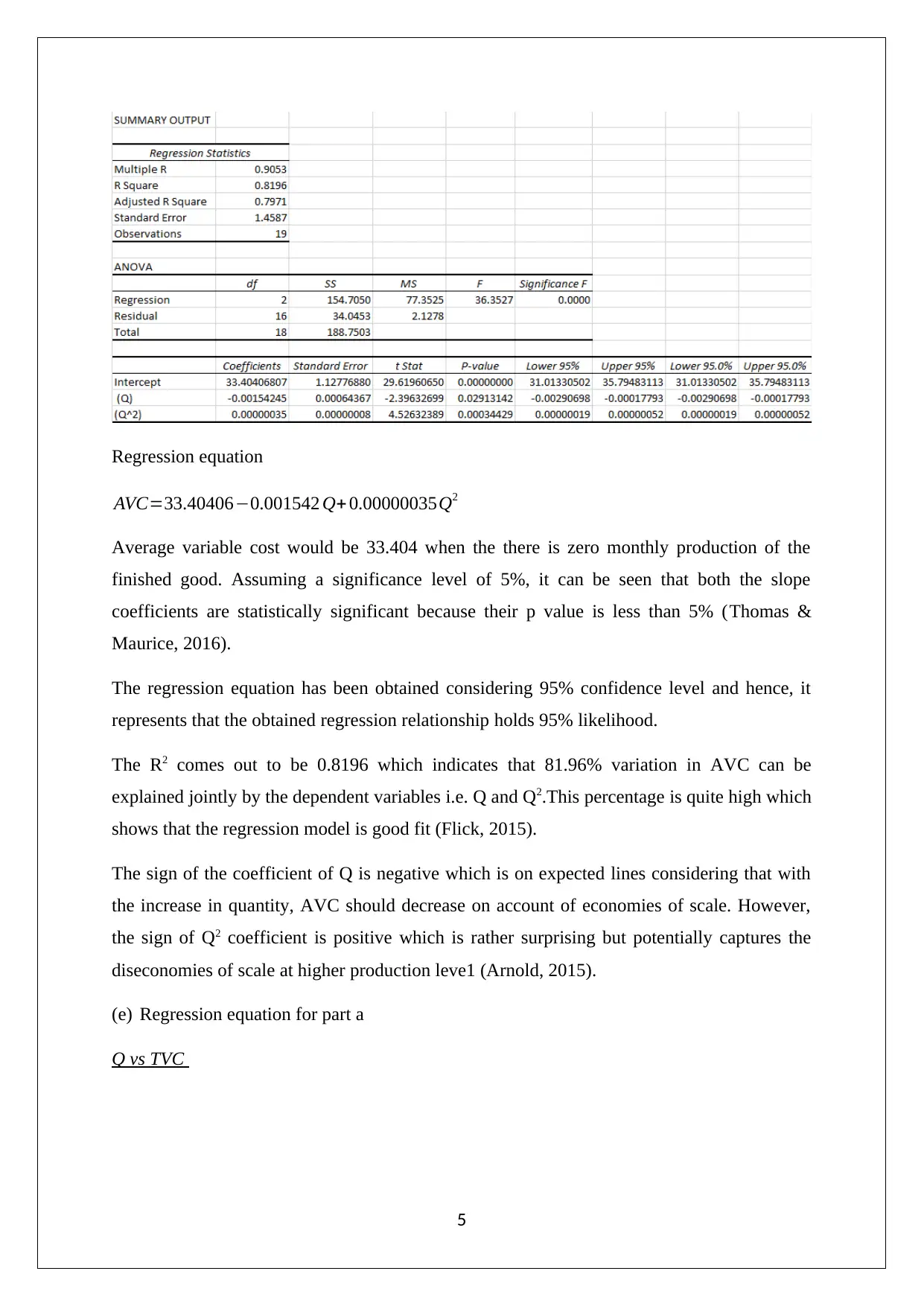
Regression equation
AVC=33.40406−0.001542 Q+ 0.00000035Q2
Average variable cost would be 33.404 when the there is zero monthly production of the
finished good. Assuming a significance level of 5%, it can be seen that both the slope
coefficients are statistically significant because their p value is less than 5% (Thomas &
Maurice, 2016).
The regression equation has been obtained considering 95% confidence level and hence, it
represents that the obtained regression relationship holds 95% likelihood.
The R2 comes out to be 0.8196 which indicates that 81.96% variation in AVC can be
explained jointly by the dependent variables i.e. Q and Q2.This percentage is quite high which
shows that the regression model is good fit (Flick, 2015).
The sign of the coefficient of Q is negative which is on expected lines considering that with
the increase in quantity, AVC should decrease on account of economies of scale. However,
the sign of Q2 coefficient is positive which is rather surprising but potentially captures the
diseconomies of scale at higher production leve1 (Arnold, 2015).
(e) Regression equation for part a
Q vs TVC
5

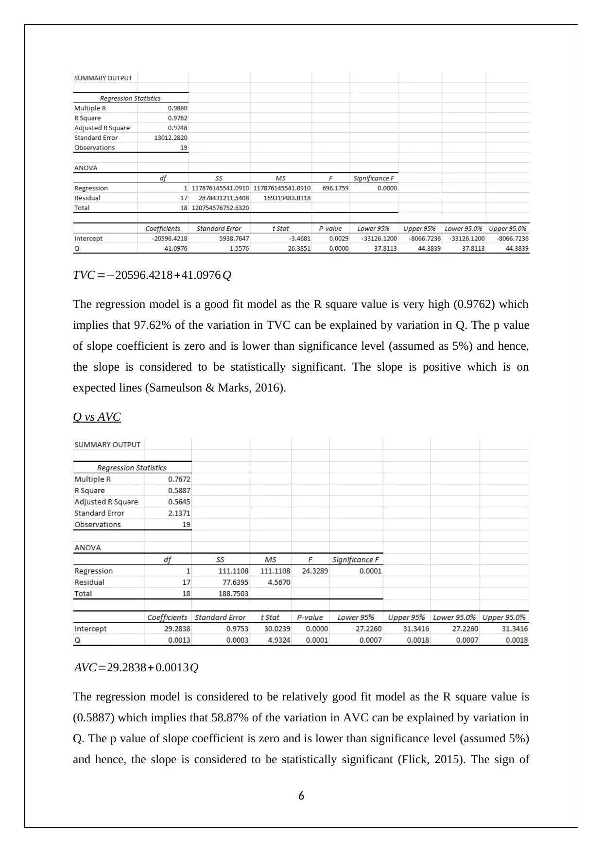
TVC =−20596.4218+41.0976 Q
The regression model is a good fit model as the R square value is very high (0.9762) which
implies that 97.62% of the variation in TVC can be explained by variation in Q. The p value
of slope coefficient is zero and is lower than significance level (assumed as 5%) and hence,
the slope is considered to be statistically significant. The slope is positive which is on
expected lines (Sameulson & Marks, 2016).
Q vs AVC
AVC=29.2838+ 0.0013Q
The regression model is considered to be relatively good fit model as the R square value is
(0.5887) which implies that 58.87% of the variation in AVC can be explained by variation in
Q. The p value of slope coefficient is zero and is lower than significance level (assumed 5%)
and hence, the slope is considered to be statistically significant (Flick, 2015). The sign of
6

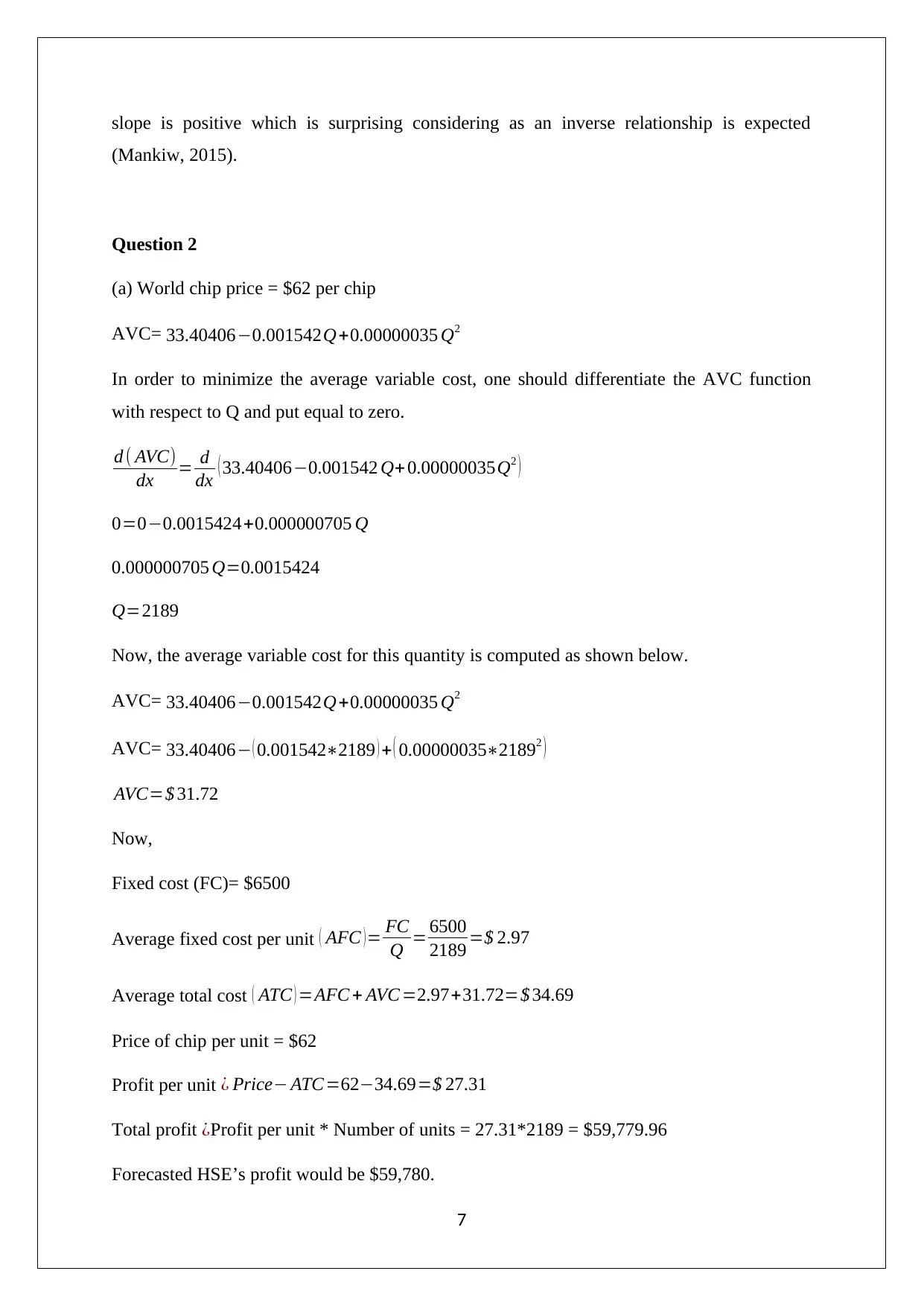
slope is positive which is surprising considering as an inverse relationship is expected
(Mankiw, 2015).
Question 2
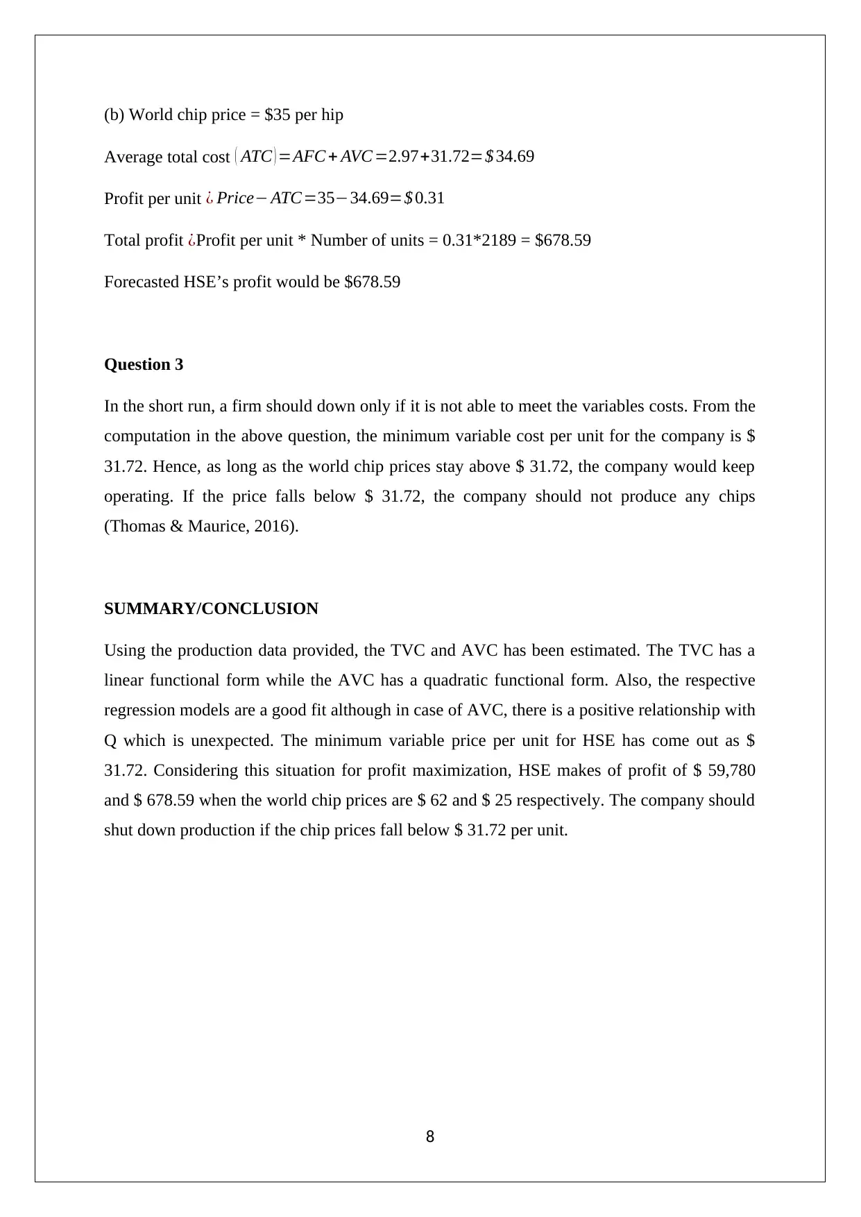
(a) World chip price = $62 per chip
AVC= 33.40406−0.001542Q+0.00000035 Q2
In order to minimize the average variable cost, one should differentiate the AVC function
with respect to Q and put equal to zero.
d ( AVC)
dx = d
dx ( 33.40406−0.001542 Q+ 0.00000035Q2 )
0=0−0.0015424+0.000000705 Q
0.000000705 Q=0.0015424
Q=2189
Now, the average variable cost for this quantity is computed as shown below.
AVC= 33.40406−0.001542Q+0.00000035 Q2
AVC= 33.40406− ( 0.001542∗2189 ) + ( 0.00000035∗21892 )
AVC=$ 31.72
Now,
Fixed cost (FC)= $6500
Average fixed cost per unit ( AFC ) = FC
Q = 6500
2189 =$ 2.97
Average total cost ( ATC ) =AFC + AVC =2.97+31.72=$ 34.69
Price of chip per unit = $62
Profit per unit ¿ Price− ATC=62−34.69=$ 27.31
Total profit ¿Profit per unit * Number of units = 27.31*2189 = $59,779.96
Forecasted HSE’s profit would be $59,780.
7

(b) World chip price = $35 per hip
Average total cost ( ATC ) =AFC + AVC =2.97+31.72=$ 34.69
Profit per unit ¿ Price− ATC=35−34.69=$ 0.31
Total profit ¿Profit per unit * Number of units = 0.31*2189 = $678.59
Forecasted HSE’s profit would be $678.59
Question 3
In the short run, a firm should down only if it is not able to meet the variables costs. From the
computation in the above question, the minimum variable cost per unit for the company is $
31.72. Hence, as long as the world chip prices stay above $ 31.72, the company would keep
operating. If the price falls below $ 31.72, the company should not produce any chips
(Thomas & Maurice, 2016).
SUMMARY/CONCLUSION
Using the production data provided, the TVC and AVC has been estimated. The TVC has a
linear functional form while the AVC has a quadratic functional form. Also, the respective
regression models are a good fit although in case of AVC, there is a positive relationship with
Q which is unexpected. The minimum variable price per unit for HSE has come out as $
31.72. Considering this situation for profit maximization, HSE makes of profit of $ 59,780
and $ 678.59 when the world chip prices are $ 62 and $ 25 respectively. The company should
shut down production if the chip prices fall below $ 31.72 per unit.
8

References
Arnold, A.R. (2015). Microeconomics (9thed.). New York, NY: Cengage Learning.
Flick, U. (2015). Introducing research methodology: A beginner's guide to doing a research
project (4thed.). New York: Sage Publications.
Mankiw, G. (2015) Microeconomics (6thed.). London: Worth Publishers.
Samuelson, W. & Marks, S. (2016). Managerial Economics (4th ed.). New York, NY: Wiley
Publications.
Thomas, C. R., & Maurice, S. C. (2016), Managerial economics: Foundations of business
analysis and strategy (12thed.). New York, NY: McGraw-Hill.
.
9