Decision Support System: Comprehensive Analysis and Project Report

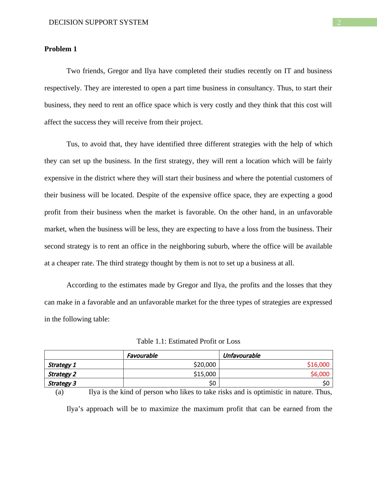
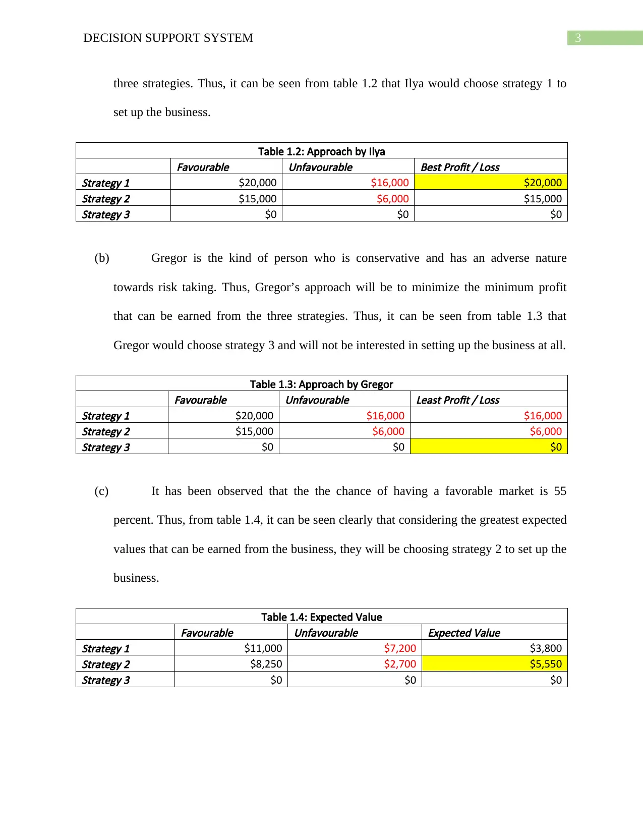
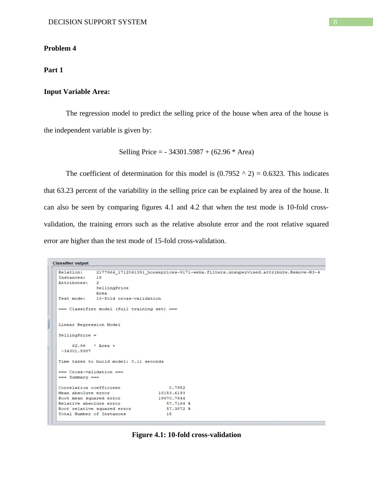
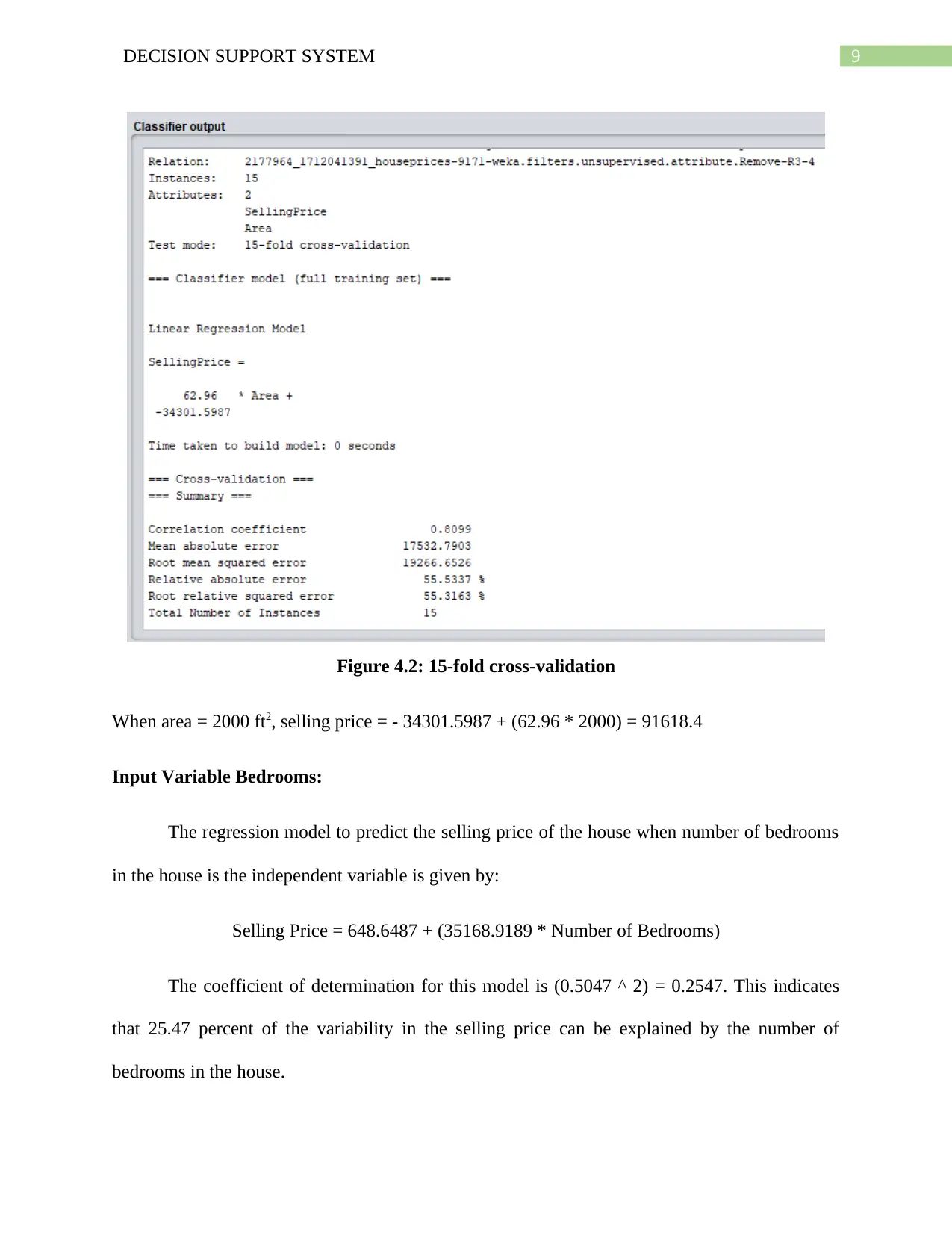
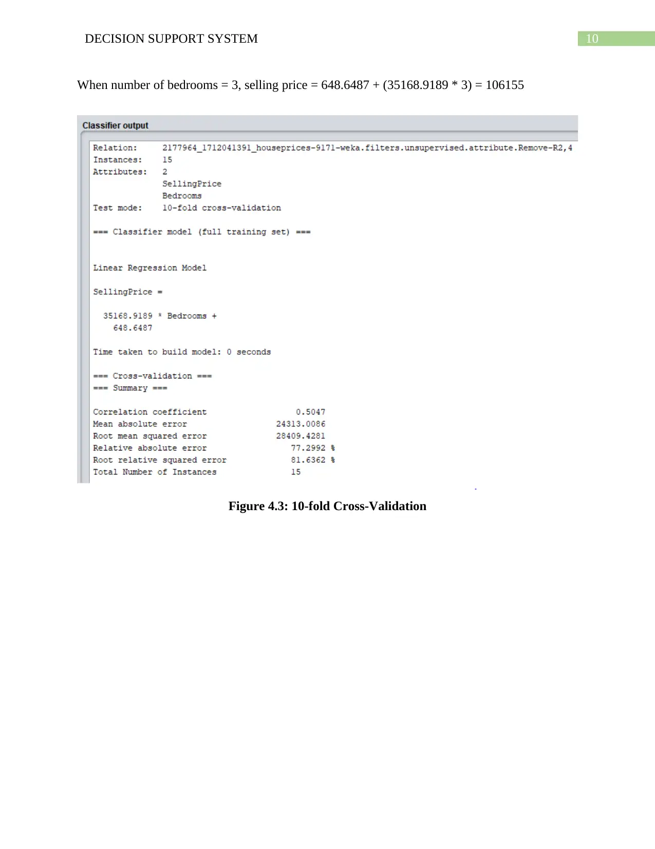
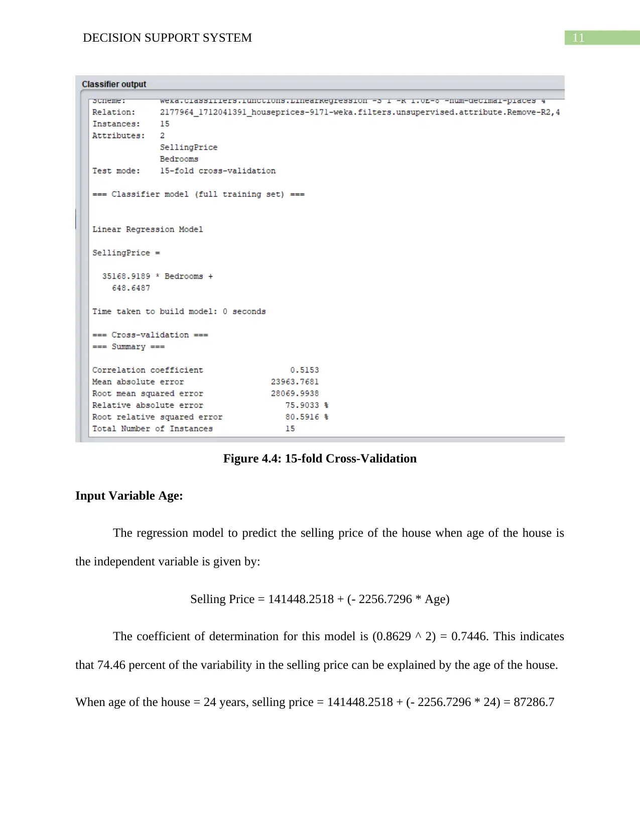
This project delves into various aspects of Decision Support Systems (DSS). It begins by analyzing a business scenario involving two friends starting a consultancy, using decision-making approaches like maximizing maximum profit and minimizing minimum profit under different market conditions. The project then formulates and solves a linear programming problem to optimize advertising budget allocation. Further, it explores inventory management through simulation, comparing different reorder point and quantity strategies to minimize costs. The core of the project involves regression analysis, predicting house selling prices using factors like area, number of bedrooms, and age. Different models are built and compared, including multiple linear regression models. Finally, the project utilizes a multilayer perceptron for prediction, evaluating its performance using the correlation coefficient. The project covers a range of DSS techniques, from optimization and simulation to predictive modeling using regression and machine learning.

Running Head: DECISION SUPPORT SYSTEM
Decision Support System
Name of the Student
Name of the University
Author Note

1DECISION SUPPORT SYSTEM
Table of Contents
Problem 1.........................................................................................................................................2
Problem 2.........................................................................................................................................5
Problem 3.........................................................................................................................................7
Problem 4.........................................................................................................................................8
Part 1............................................................................................................................................8
Part 2..........................................................................................................................................13
Problem 5.......................................................................................................................................21
Problem 6.......................................................................................................................................22
Task 1.........................................................................................................................................22
Task 2.........................................................................................................................................24
Conclusion.................................................................................................................................26

2DECISION SUPPORT SYSTEM
Problem 1
Two friends, Gregor and Ilya have completed their studies recently on IT and business
respectively. They are interested to open a part time business in consultancy. Thus, to start their
business, they need to rent an office space which is very costly and they think that this cost will
affect the success they will receive from their project.
Tus, to avoid that, they have identified three different strategies with the help of which
they can set up the business. In the first strategy, they will rent a location which will be fairly
expensive in the district where they will start their business and where the potential customers of
their business will be located. Despite of the expensive office space, they are expecting a good
profit from their business when the market is favorable. On the other hand, in an unfavorable
market, when the business will be less, they are expecting to have a loss from the business. Their
second strategy is to rent an office in the neighboring suburb, where the office will be available
at a cheaper rate. The third strategy thought by them is not to set up a business at all.
According to the estimates made by Gregor and Ilya, the profits and the losses that they
can make in a favorable and an unfavorable market for the three types of strategies are expressed
in the following table:
Table 1.1: Estimated Profit or Loss
Favourable
Unfavourable
Strategy 1 $20,000 $16,000
Strategy 2 $15,000 $6,000
Strategy 3 $0 $0
(a) Ilya is the kind of person who likes to take risks and is optimistic in nature. Thus,
Ilya’s approach will be to maximize the maximum profit that can be earned from the

3DECISION SUPPORT SYSTEM
three strategies. Thus, it can be seen from table 1.2 that Ilya would choose strategy 1 to
set up the business.
Table 1.2: Approach by Ilya
Favourable
Unfavourable
Best Profit / Loss
Strategy 1 $20,000 $16,000 $20,000
Strategy 2 $15,000 $6,000 $15,000
Strategy 3 $0 $0 $0
(b) Gregor is the kind of person who is conservative and has an adverse nature
towards risk taking. Thus, Gregor’s approach will be to minimize the minimum profit
that can be earned from the three strategies. Thus, it can be seen from table 1.3 that
Gregor would choose strategy 3 and will not be interested in setting up the business at all.
Table 1.3: Approach by Gregor
Favourable
Unfavourable
Least Profit / Loss
Strategy 1 $20,000 $16,000 $16,000
Strategy 2 $15,000 $6,000 $6,000
Strategy 3 $0 $0 $0
(c) It has been observed that the the chance of having a favorable market is 55
percent. Thus, from table 1.4, it can be seen clearly that considering the greatest expected
values that can be earned from the business, they will be choosing strategy 2 to set up the
business.
Table 1.4: Expected Value
Favourable
Unfavourable
Expected Value
Strategy 1 $11,000 $7,200 $3,800
Strategy 2 $8,250 $2,700 $5,550
Strategy 3 $0 $0 $0

4DECISION SUPPORT SYSTEM
(d) The plot showing the expected values of returns from strategy 1 and strategy 2 is
given in figure 1.1 when the probability of favorable market varies from 0 to 1.
0.00 0.20 0.40 0.60 0.80 1.00 1.20
$20,000
$15,000
$10,000
$5,000
$0
$5,000
$10,000
$15,000
$20,000
$25,000
Expected Returns of Strategy 1 and Strategy 2
Strategy 1
Strategy 2
Probability
Expected Values
Figure 1.1: Expected returns from Strategy 1 and Strategy 2
(e) i) It can be seen from the graph that expected returns from strategy 1 is higher than
strategy 2 and strategy 3 when the probability of favorable market is more than 0.66.
Thus, Strategy 1 will be selected when 0.67 ≤ P ≤ 1
ii) It can be seen from the graph that expected returns from strategy 2 is higher than
strategy 1 and strategy 3 when the probability of favorable market is between 0.29 and
0.66. Thus, Strategy 2 will be selected when 0.29 ≤ P ≤ 0.66
iii) It can be seen from the graph that both strategy 1 and strategy 2 face loses in the
expected returns when the probability of favorable market is less than 0.28. Thus,
Strategy 3 will be selected. Thus, Strategy 3 will be selected when 0 ≤ P ≤ 0.28

5DECISION SUPPORT SYSTEM
Problem 2
Let the number of TV ads be x1, radio ads be x2, billboard ads be x3 and newspaper ads be
x4.
Minimize Z = 960 x1 + 480 x2 + 600 x3 + 120 x4
Subject to the constraints:
x1 ≤ 10
x2 ≤ 10
x3 ≤ 10
x4 ≤ 10
x1 ≥ 10
x2 ≥ 10
x1 + x2 ≥ 6
960 x1 – 600 x3 – 120 x4 ≥ 0
And the non-negativity constraints x1 ≥ 0, x2 ≥ 0, x3 ≥ 0, x4 ≥ 0

6DECISION SUPPORT SYSTEM
(a) The maximum number of people that can reach on his weekly budget of $14,000
is (6 * 36,000) + (6 * 26,500) = 3,75,000
(b) He must order 6 TV ads and 6 Radio ads in order to receive this result.

7DECISION SUPPORT SYSTEM
Problem 3
(a) It can be seen as a result of the simulation conducted that the least cost of
inventory policy acquired by Max is $43,380, which is the best case. The Highest cost
that can be acquired by Max is $63,060. This is the worst case. On an average, it is
expected that Max will incur a cost of $56, 030 on the inventory policy.
(b) i) Considering the re-order point as 3 and the reordering quantity as 3, it can be seen
as a result of the simulation conducted that the least cost of inventory policy acquired by
Max is $27,120, which is the best case. The Highest cost that can be acquired by Max is
$42,420. This is the worst case. On an average, it is expected that Max will incur a cost of
$35,976 on the inventory policy.
ii) Considering the re-order point as 7 and the reordering quantity as 7, it can be seen
as a result of the simulation conducted that the least cost of inventory policy acquired by
Max is $78,260, which is the best case. The Highest cost that can be acquired by Max is
$1,09,520. This is the worst case. On an average, it is expected that Max will incur a cost
of $90,544 on the inventory policy.
(c) From the discussion conducted above, it can be seen clearly that with a reordering
point of 3 and reordering quantity of 3, the average cost incurred for inventory policy is
less than the situation when the re-order point as 7 and the reordering quantity as 7. Thus,
reordering point of 3 and reordering quantity of 3 will be a better policy to run the
business.

8DECISION SUPPORT SYSTEM
Problem 4
Part 1
Input Variable Area:
The regression model to predict the selling price of the house when area of the house is
the independent variable is given by:
Selling Price = - 34301.5987 + (62.96 * Area)
The coefficient of determination for this model is (0.7952 ^ 2) = 0.6323. This indicates
that 63.23 percent of the variability in the selling price can be explained by area of the house. It
can also be seen by comparing figures 4.1 and 4.2 that when the test mode is 10-fold cross-
validation, the training errors such as the relative absolute error and the root relative squared
error are higher than the test mode of 15-fold cross-validation.
Figure 4.1: 10-fold cross-validation

9DECISION SUPPORT SYSTEM
Figure 4.2: 15-fold cross-validation
When area = 2000 ft2, selling price = - 34301.5987 + (62.96 * 2000) = 91618.4
Input Variable Bedrooms:
The regression model to predict the selling price of the house when number of bedrooms
in the house is the independent variable is given by:
Selling Price = 648.6487 + (35168.9189 * Number of Bedrooms)
The coefficient of determination for this model is (0.5047 ^ 2) = 0.2547. This indicates
that 25.47 percent of the variability in the selling price can be explained by the number of
bedrooms in the house.

10DECISION SUPPORT SYSTEM
When number of bedrooms = 3, selling price = 648.6487 + (35168.9189 * 3) = 106155
Figure 4.3: 10-fold Cross-Validation

11DECISION SUPPORT SYSTEM
Figure 4.4: 15-fold Cross-Validation
Input Variable Age:
The regression model to predict the selling price of the house when age of the house is
the independent variable is given by:
Selling Price = 141448.2518 + (- 2256.7296 * Age)
The coefficient of determination for this model is (0.8629 ^ 2) = 0.7446. This indicates
that 74.46 percent of the variability in the selling price can be explained by the age of the house.
When age of the house = 24 years, selling price = 141448.2518 + (- 2256.7296 * 24) = 87286.7