CSE5DSS: Decision Support System Project - Data Analysis and Modeling

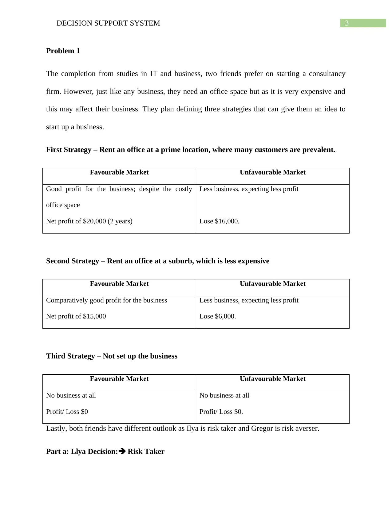
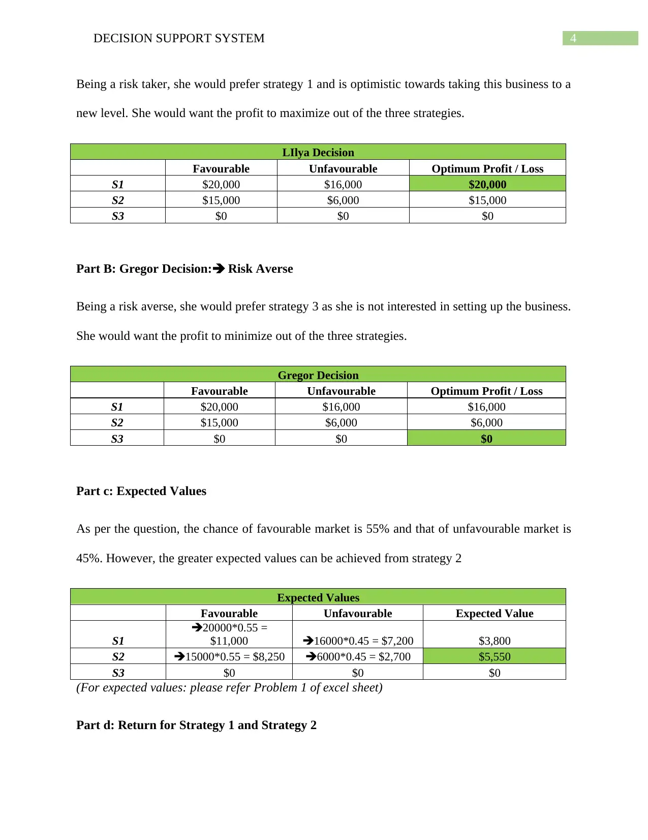
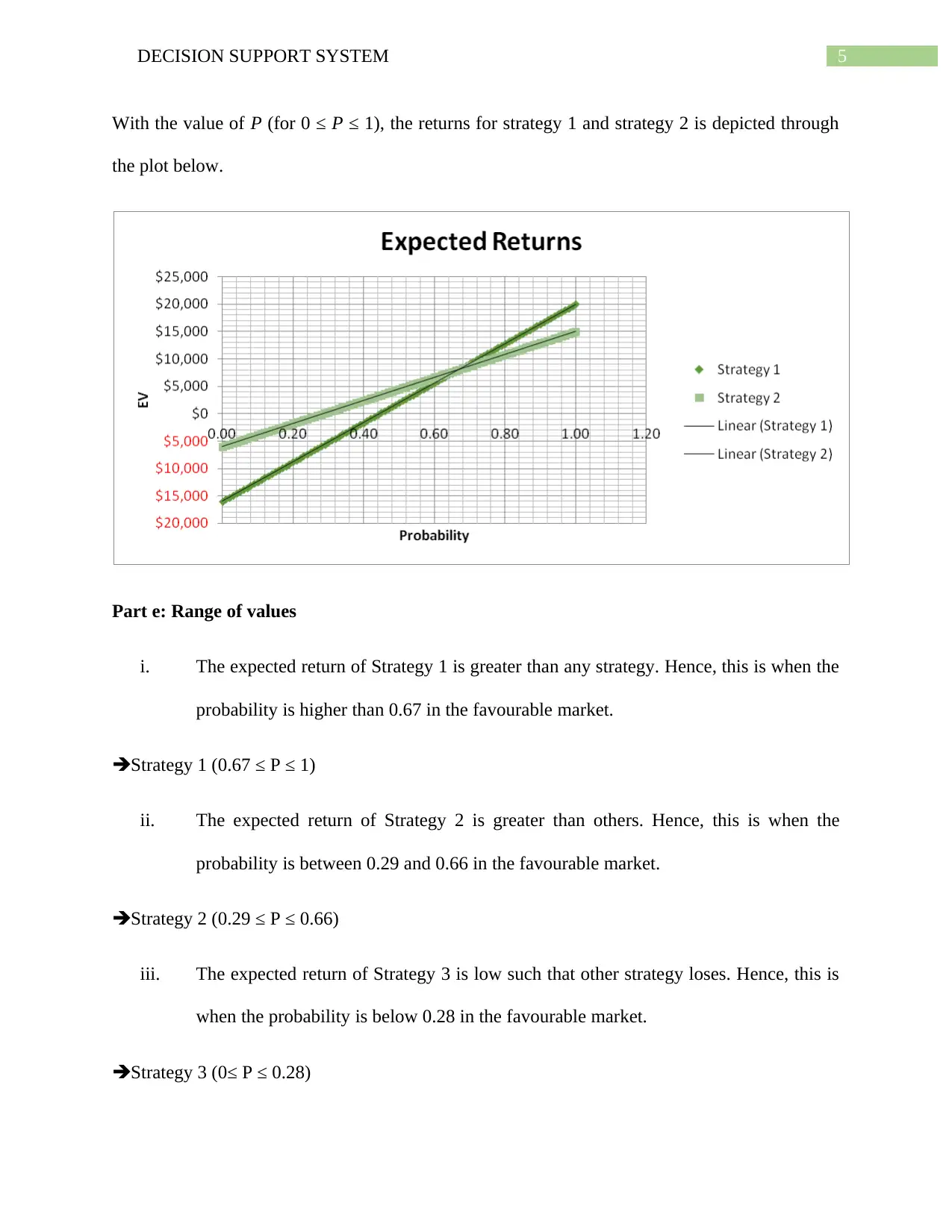
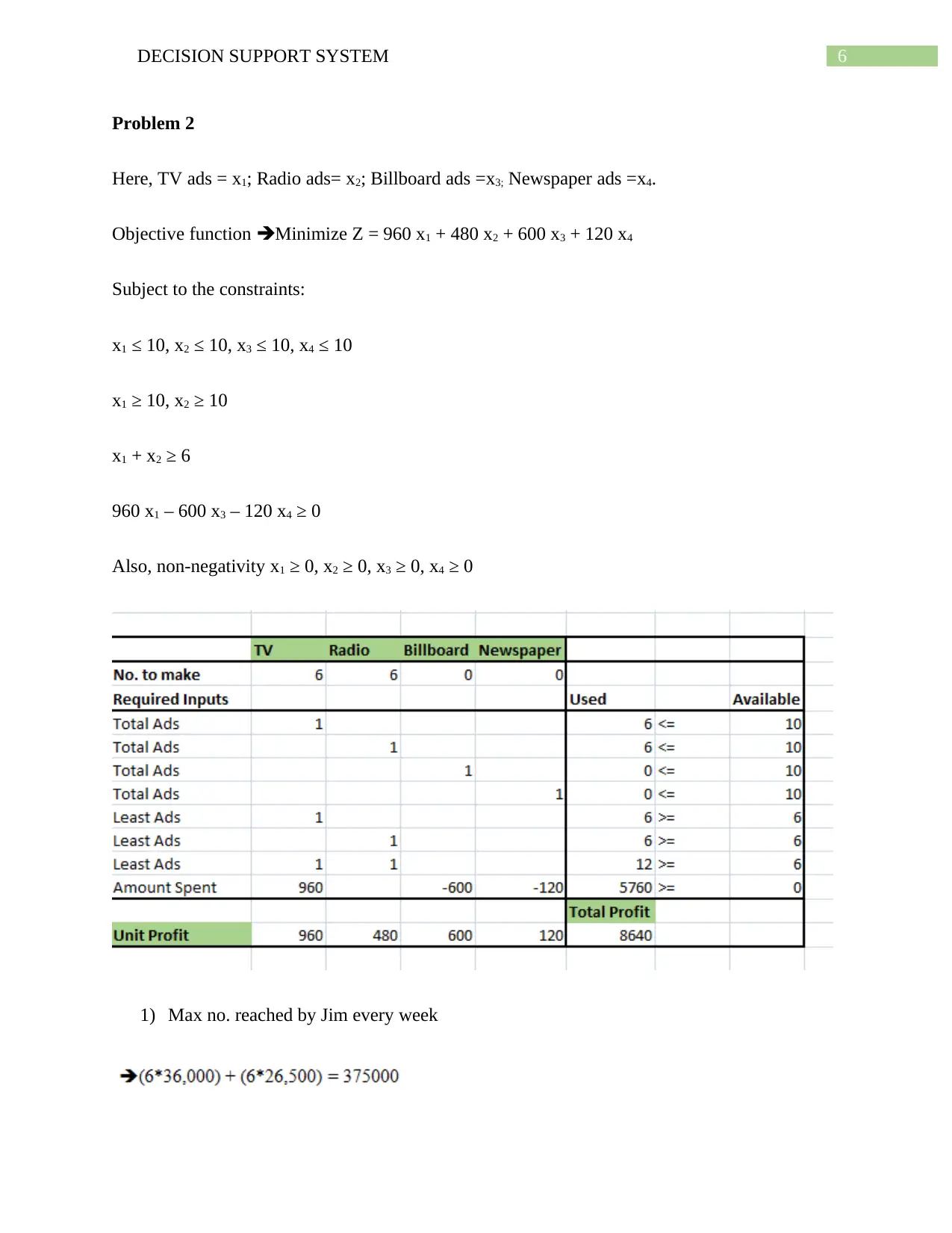
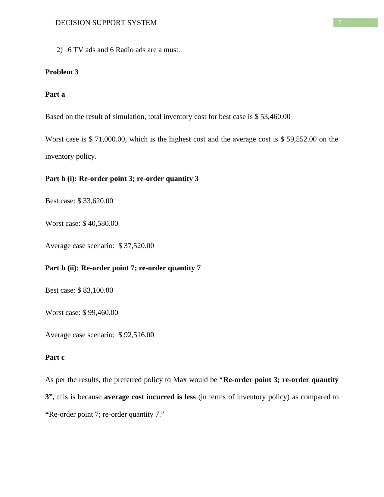
This project analyzes a Decision Support System (DSS) through various problems and tasks. Problem 1 explores decision-making under uncertainty using expected values and different strategies for business start-up, including risk-taking and risk-averse scenarios. Problem 2 formulates a linear programming problem for advertising optimization. Problem 3 analyzes inventory management using simulation. Problem 4 focuses on predicting house prices using regression models with different input variables and multiple regression techniques. Problem 5 uses Multi-Layer Perceptrons (MLPs) for house price prediction and compares their performance. Problem 6 and Task 1 delve into classification models, including logistic regression and Naive Bayes, evaluating their performance using confusion matrices, ROC curves, and area under ROC. Task 2 presents lift charts for both models. The project concludes by comparing the performance of the classifiers and providing insights into the best-performing models for the given datasets. The project covers various data science and machine learning techniques to solve the decision support system problems.

Running Head: DECISION SUPPORT SYSTEM
CSE5DSS – Decision Support System
Name of the Student
Student Id:

1DECISION SUPPORT SYSTEM
Table of Contents
Problem 1.........................................................................................................................................3
Part a: Llya Decision: Risk Taker............................................................................................3
Part B: Gregor Decision: Risk Averse.....................................................................................4
Part c: Expected Values...............................................................................................................4
Part d: Return for Strategy 1 and Strategy 2................................................................................4
Part e: Range of values................................................................................................................5
Problem 2.........................................................................................................................................6
Problem 3.........................................................................................................................................7
Part a............................................................................................................................................7
Part b (i): Re-order point 3; re-order quantity 3..........................................................................7
Part b (ii): Re-order point 7; re-order quantity 7.........................................................................7
Part c............................................................................................................................................7
Problem 4.........................................................................................................................................8
Part 1............................................................................................................................................8
Part 2..........................................................................................................................................12
Problem 5.......................................................................................................................................19
Problem 6.......................................................................................................................................21
Preliminary questions................................................................................................................21
Task 1.........................................................................................................................................21

2DECISION SUPPORT SYSTEM
I. Logistic Regression............................................................................................................21
Part a: Confusion Matrix...........................................................................................................21
Part b: ROC Curve.....................................................................................................................21
Part c: Area under ROC Curve..................................................................................................22
II. Naïve Bayes Model.........................................................................................................22
Part a: Confusion Matrix...........................................................................................................22
Part b: ROC Curve.....................................................................................................................22
Part c: Area under ROC Curve..................................................................................................23
Task 2.........................................................................................................................................23
Lift Chart for Logistic Regression Model.................................................................................23
Lift Chart for Naïve Bayes Model.............................................................................................24
Conclusion.................................................................................................................................25

3DECISION SUPPORT SYSTEM
Problem 1
The completion from studies in IT and business, two friends prefer on starting a consultancy
firm. However, just like any business, they need an office space but as it is very expensive and
this may affect their business. They plan defining three strategies that can give them an idea to
start up a business.
First Strategy – Rent an office at a prime location, where many customers are prevalent.
Favourable Market Unfavourable Market
Good profit for the business; despite the costly
office space
Net profit of $20,000 (2 years)
Less business, expecting less profit
Lose $16,000.
Second Strategy – Rent an office at a suburb, which is less expensive
Favourable Market Unfavourable Market
Comparatively good profit for the business
Net profit of $15,000
Less business, expecting less profit
Lose $6,000.
Third Strategy – Not set up the business
Favourable Market Unfavourable Market
No business at all
Profit/ Loss $0
No business at all
Profit/ Loss $0.
Lastly, both friends have different outlook as Ilya is risk taker and Gregor is risk averser.
Part a: Llya Decision: Risk Taker

4DECISION SUPPORT SYSTEM
Being a risk taker, she would prefer strategy 1 and is optimistic towards taking this business to a
new level. She would want the profit to maximize out of the three strategies.
LIlya Decision
Favourable Unfavourable Optimum Profit / Loss
S1 $20,000 $16,000 $20,000
S2 $15,000 $6,000 $15,000
S3 $0 $0 $0
Part B: Gregor Decision: Risk Averse
Being a risk averse, she would prefer strategy 3 as she is not interested in setting up the business.
She would want the profit to minimize out of the three strategies.
Gregor Decision
Favourable Unfavourable Optimum Profit / Loss
S1 $20,000 $16,000 $16,000
S2 $15,000 $6,000 $6,000
S3 $0 $0 $0
Part c: Expected Values
As per the question, the chance of favourable market is 55% and that of unfavourable market is
45%. However, the greater expected values can be achieved from strategy 2
Expected Values
Favourable Unfavourable Expected Value
S1
20000*0.55 =
$11,000 16000*0.45 = $7,200 $3,800
S2 15000*0.55 = $8,250 6000*0.45 = $2,700 $5,550
S3 $0 $0 $0
(For expected values: please refer Problem 1 of excel sheet)
Part d: Return for Strategy 1 and Strategy 2

5DECISION SUPPORT SYSTEM
With the value of P (for 0 ≤ P ≤ 1), the returns for strategy 1 and strategy 2 is depicted through
the plot below.
Part e: Range of values
i. The expected return of Strategy 1 is greater than any strategy. Hence, this is when the
probability is higher than 0.67 in the favourable market.
Strategy 1 (0.67 ≤ P ≤ 1)
ii. The expected return of Strategy 2 is greater than others. Hence, this is when the
probability is between 0.29 and 0.66 in the favourable market.
Strategy 2 (0.29 ≤ P ≤ 0.66)
iii. The expected return of Strategy 3 is low such that other strategy loses. Hence, this is
when the probability is below 0.28 in the favourable market.
Strategy 3 (0≤ P ≤ 0.28)

6DECISION SUPPORT SYSTEM
Problem 2
Here, TV ads = x1; Radio ads= x2; Billboard ads =x3; Newspaper ads =x4.
Objective function Minimize Z = 960 x1 + 480 x2 + 600 x3 + 120 x4
Subject to the constraints:
x1 ≤ 10, x2 ≤ 10, x3 ≤ 10, x4 ≤ 10
x1 ≥ 10, x2 ≥ 10
x1 + x2 ≥ 6
960 x1 – 600 x3 – 120 x4 ≥ 0
Also, non-negativity x1 ≥ 0, x2 ≥ 0, x3 ≥ 0, x4 ≥ 0
1) Max no. reached by Jim every week

7DECISION SUPPORT SYSTEM
2) 6 TV ads and 6 Radio ads are a must.
Problem 3
Part a
Based on the result of simulation, total inventory cost for best case is $ 53,460.00
Worst case is $ 71,000.00, which is the highest cost and the average cost is $ 59,552.00 on the
inventory policy.
Part b (i): Re-order point 3; re-order quantity 3
Best case: $ 33,620.00
Worst case: $ 40,580.00
Average case scenario: $ 37,520.00
Part b (ii): Re-order point 7; re-order quantity 7
Best case: $ 83,100.00
Worst case: $ 99,460.00
Average case scenario: $ 92,516.00
Part c
As per the results, the preferred policy to Max would be “Re-order point 3; re-order quantity
3”, this is because average cost incurred is less (in terms of inventory policy) as compared to
“Re-order point 7; re-order quantity 7.”

8DECISION SUPPORT SYSTEM
Problem 4
Part 1
Model 1
Predicting the selling price by using area of house
SP = - 34301.5987 + 62.96*Area_of_house
“Leave one out cross validation error = 18153.6193”
Coefficient of determination = 0.7952 ^ 2 = 0.6323. This suggests that 63.23% variation in the
model can be explained by area of the house.
The 10 fold cross validation, the errors like training error (relative absolute+ root relative)
squared are higher than test mode of 15-fold cross-validation
Figure: “10-fold cross-validation”

9DECISION SUPPORT SYSTEM
Figure: “15-fold cross-validation”
Hence, Area = 2000 ft2, “SP = - 34301.5987 + (62.96*2000) = 91618.4”
Model 2
Predicting the selling price by using no. of bedrooms
SP= 648.6487 + 35168.9189*No._of_Bedrooms
“Leave one out cross validation error = 24313.0086”
Coefficient of determination = 0.5047 ^ 2 = 0.2547. This suggests that 25.47% variation in the
model can be explained by no. of bedrooms.

10DECISION SUPPORT SYSTEM
Figure: “10-fold cross-validation”

11DECISION SUPPORT SYSTEM
Figure: “15-fold cross-validation”
Hence, no. of bedrooms = 3, “SP = 648.6487 + (35168.9189 * 3) = 106155”
Model 3
Predicting the selling price by using age as an input
SP= 141448.2518 - 2256.7296*Age
“Leave one out cross validation error = 24313.0086”
Coefficient of determination = 0.8629 ^ 2 = 0.7446. This suggests that 74.46% variation in the
model can be explained by age of the house.
Figure: “10-fold cross-validation”