Break-Even Analysis and Product Mix

This assignment focuses on break-even analysis for two products (A and B) with varying sale prices and variable costs. Students calculate the breakeven point in units for each product, determine the required sales volume based on a given sales mix ratio, and then analyze the total sales needed to achieve a specific profit target.

DECISION SUPPORT TOOLS
STUDENT ID:
[Pick the date]

Question 1
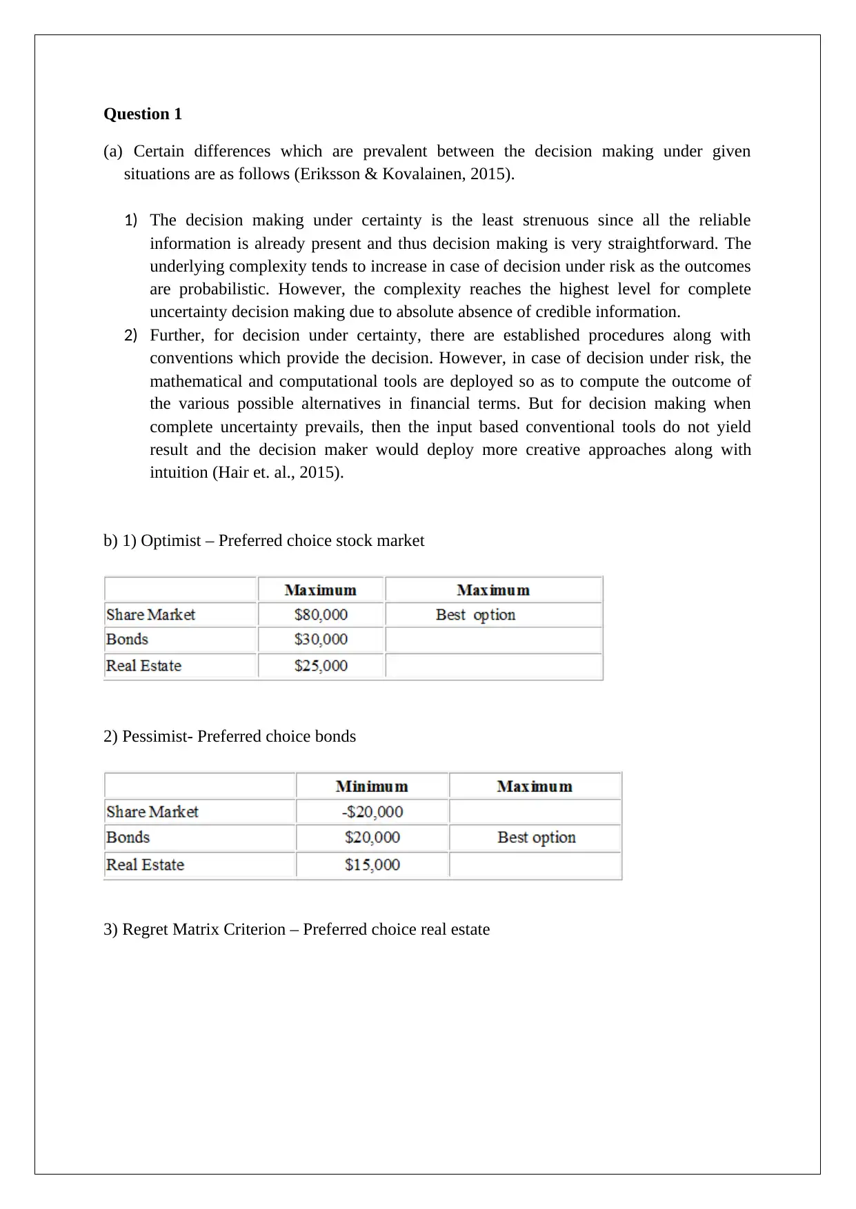
(a) Certain differences which are prevalent between the decision making under given
situations are as follows (Eriksson & Kovalainen, 2015).
1) The decision making under certainty is the least strenuous since all the reliable
information is already present and thus decision making is very straightforward. The
underlying complexity tends to increase in case of decision under risk as the outcomes
are probabilistic. However, the complexity reaches the highest level for complete
uncertainty decision making due to absolute absence of credible information.
2) Further, for decision under certainty, there are established procedures along with
conventions which provide the decision. However, in case of decision under risk, the
mathematical and computational tools are deployed so as to compute the outcome of
the various possible alternatives in financial terms. But for decision making when
complete uncertainty prevails, then the input based conventional tools do not yield
result and the decision maker would deploy more creative approaches along with
intuition (Hair et. al., 2015).
b) 1) Optimist – Preferred choice stock market
2) Pessimist- Preferred choice bonds
3) Regret Matrix Criterion – Preferred choice real estate

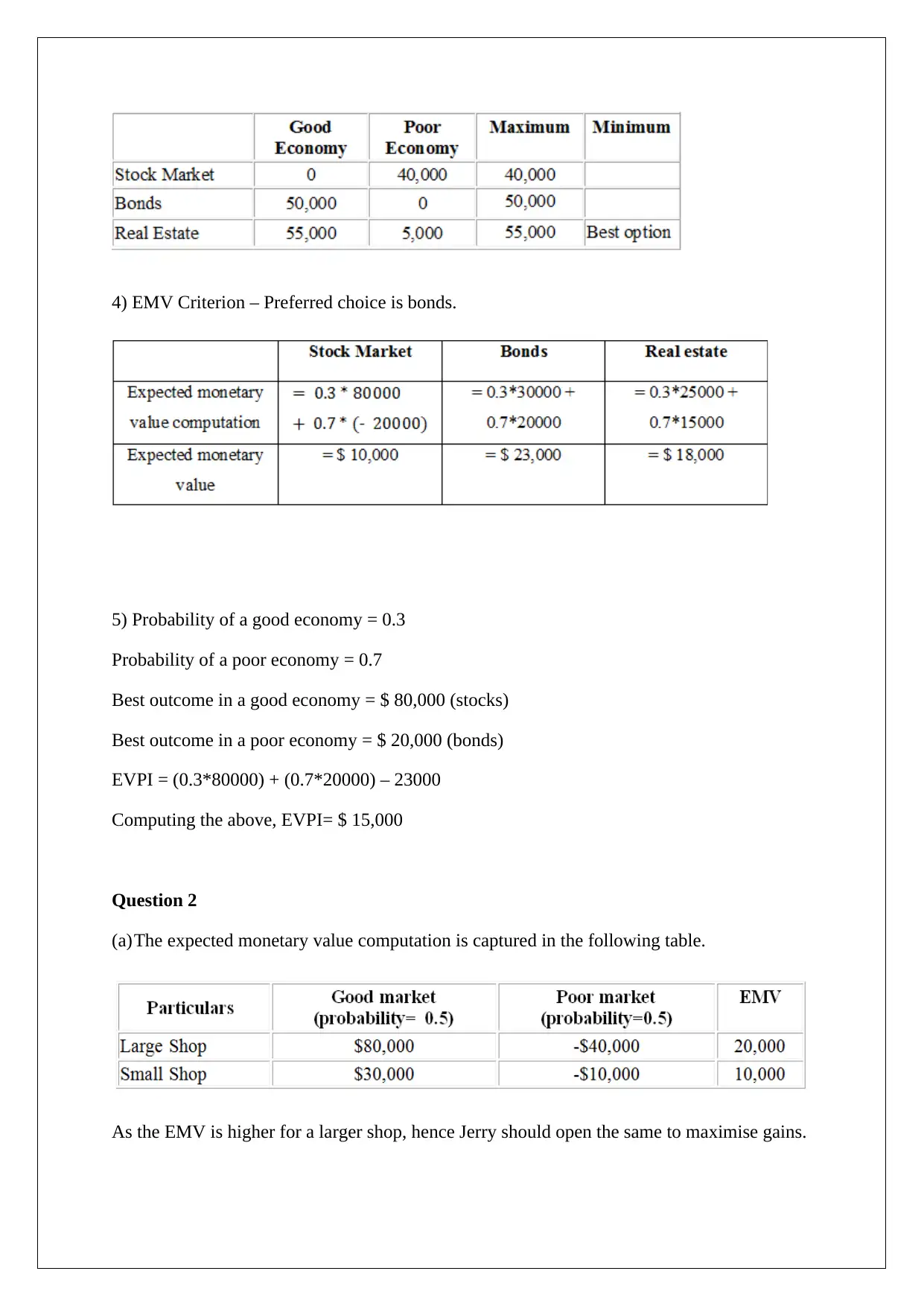
4) EMV Criterion – Preferred choice is bonds.
5) Probability of a good economy = 0.3
Probability of a poor economy = 0.7
Best outcome in a good economy = $ 80,000 (stocks)
Best outcome in a poor economy = $ 20,000 (bonds)
EVPI = (0.3*80000) + (0.7*20000) – 23000
Computing the above, EVPI= $ 15,000
Question 2
(a)The expected monetary value computation is captured in the following table.
As the EMV is higher for a larger shop, hence Jerry should open the same to maximise gains.

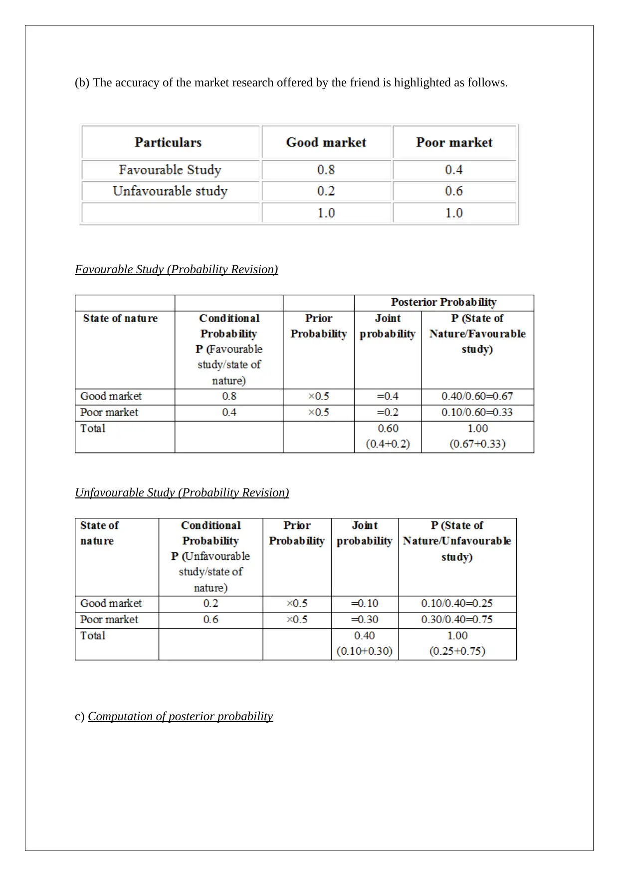
(b) The accuracy of the market research offered by the friend is highlighted as follows.
Favourable Study (Probability Revision)
Unfavourable Study (Probability Revision)
c) Computation of posterior probability

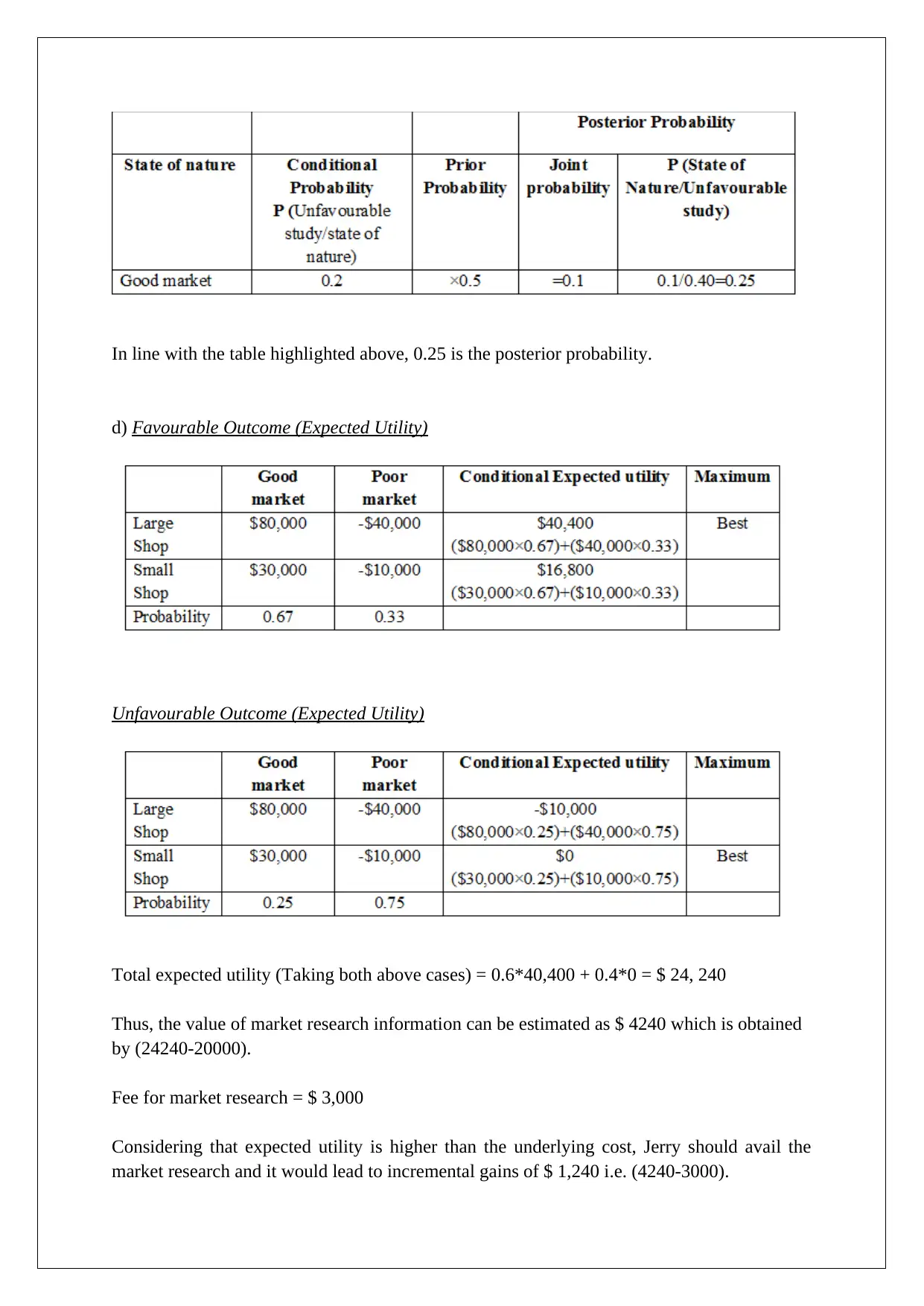
In line with the table highlighted above, 0.25 is the posterior probability.
d) Favourable Outcome (Expected Utility)
Unfavourable Outcome (Expected Utility)
Total expected utility (Taking both above cases) = 0.6*40,400 + 0.4*0 = $ 24, 240
Thus, the value of market research information can be estimated as $ 4240 which is obtained
by (24240-20000).
Fee for market research = $ 3,000
Considering that expected utility is higher than the underlying cost, Jerry should avail the
market research and it would lead to incremental gains of $ 1,240 i.e. (4240-3000).

Question 3
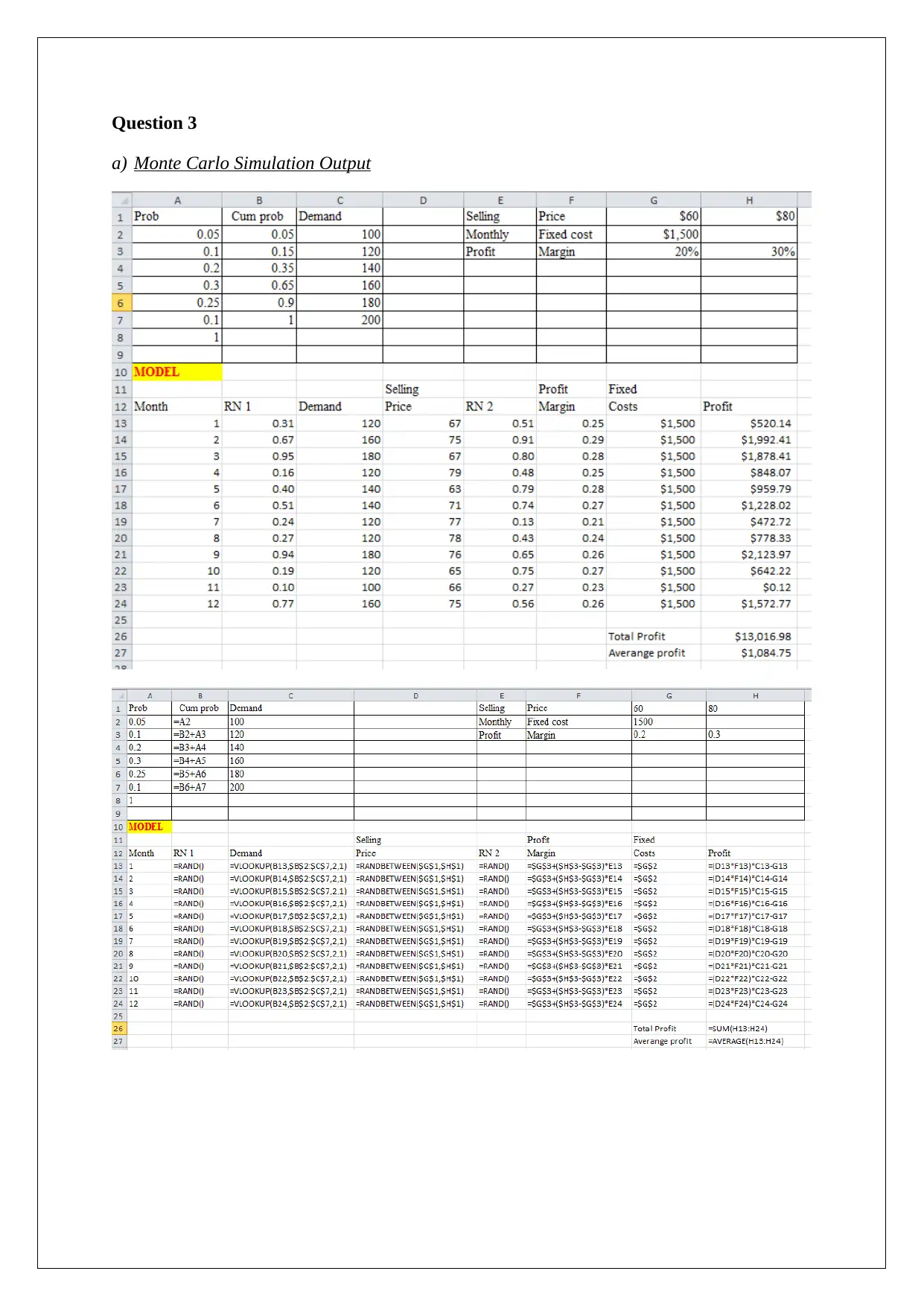
a) Monte Carlo Simulation Output

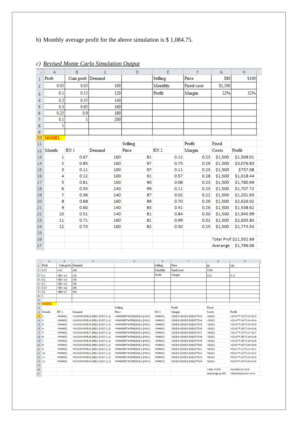
b) Monthly average profit for the above simulation is $ 1,084.75.
c) Revised Monte Carlo Simulation Output

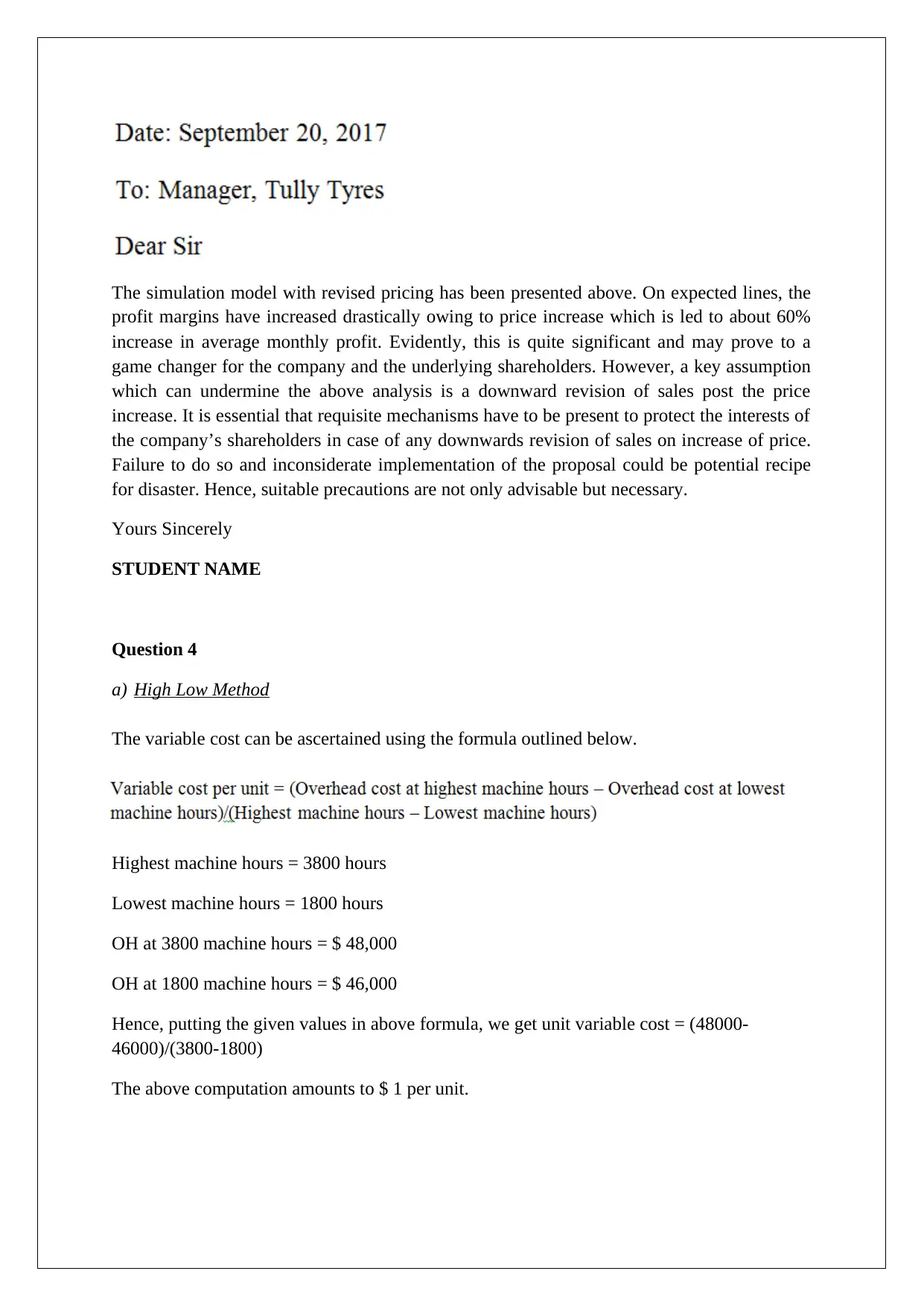
The simulation model with revised pricing has been presented above. On expected lines, the
profit margins have increased drastically owing to price increase which is led to about 60%
increase in average monthly profit. Evidently, this is quite significant and may prove to a
game changer for the company and the underlying shareholders. However, a key assumption
which can undermine the above analysis is a downward revision of sales post the price
increase. It is essential that requisite mechanisms have to be present to protect the interests of
the company’s shareholders in case of any downwards revision of sales on increase of price.
Failure to do so and inconsiderate implementation of the proposal could be potential recipe
for disaster. Hence, suitable precautions are not only advisable but necessary.
Yours Sincerely
STUDENT NAME
Question 4
a) High Low Method
The variable cost can be ascertained using the formula outlined below.
Highest machine hours = 3800 hours
Lowest machine hours = 1800 hours
OH at 3800 machine hours = $ 48,000
OH at 1800 machine hours = $ 46,000
Hence, putting the given values in above formula, we get unit variable cost = (48000-
46000)/(3800-1800)
The above computation amounts to $ 1 per unit.

Taking any given data into consideration, by substituting the variable cost, the fixed cost may
be ascertained.
When machine hours = 3800, then total overhead costs = $ 48,000
As a result, the fixed cost = 48000 – 3800*1
The above computation amounts to $ 44,200.
Hence, the derived regression equation from high low is as written below.
OH = 44200 + MH
Given that MH= 3000 hours
Therefore, overhead cost estimated = 44200 + 3000 = $ 47,200
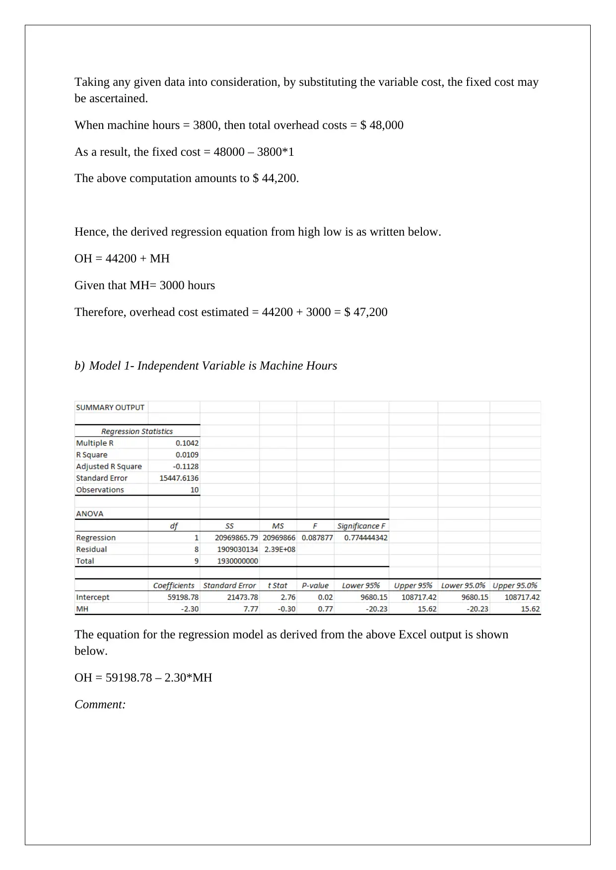
b) Model 1- Independent Variable is Machine Hours
The equation for the regression model as derived from the above Excel output is shown
below.
OH = 59198.78 – 2.30*MH
Comment:

Further, the ANOVA testing (P value > 0.05) along with the coefficient of determination
(Very Low) also hint towards model not representing a good fit (Halhn & Doganaksoy,
2011).
Model 2- Independent variable is batches
The equation for the regression model as derived from the above Excel output is shown
below.
OH = 6555.56 + 234.57* Batches
Comment:

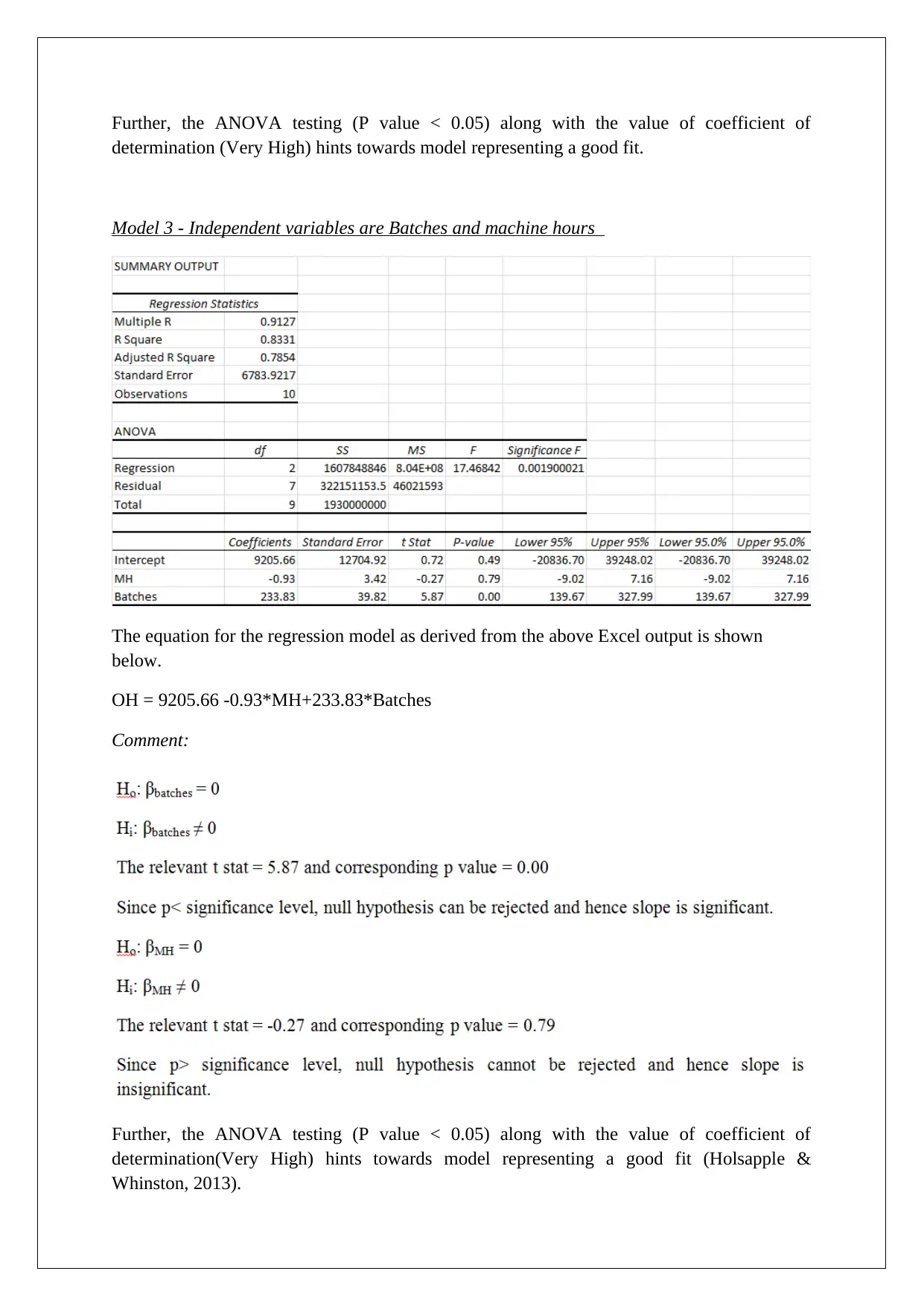
Further, the ANOVA testing (P value < 0.05) along with the value of coefficient of
determination (Very High) hints towards model representing a good fit.
Model 3 - Independent variables are Batches and machine hours
The equation for the regression model as derived from the above Excel output is shown
below.
OH = 9205.66 -0.93*MH+233.83*Batches
Comment:
Further, the ANOVA testing (P value < 0.05) along with the value of coefficient of
determination(Very High) hints towards model representing a good fit (Holsapple &
Whinston, 2013).

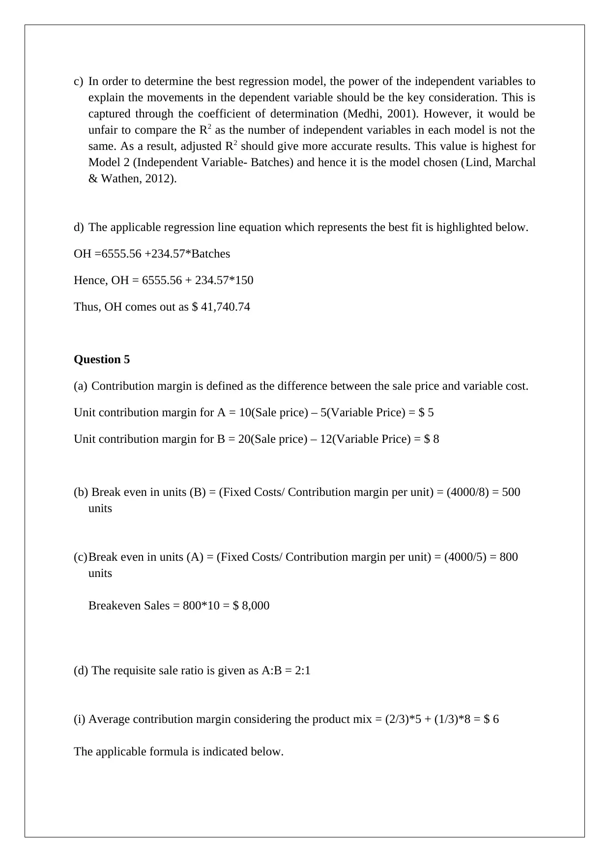
c) In order to determine the best regression model, the power of the independent variables to
explain the movements in the dependent variable should be the key consideration. This is
captured through the coefficient of determination (Medhi, 2001). However, it would be
unfair to compare the R2 as the number of independent variables in each model is not the
same. As a result, adjusted R2 should give more accurate results. This value is highest for
Model 2 (Independent Variable- Batches) and hence it is the model chosen (Lind, Marchal
& Wathen, 2012).
d) The applicable regression line equation which represents the best fit is highlighted below.
OH =6555.56 +234.57*Batches
Hence, OH = 6555.56 + 234.57*150
Thus, OH comes out as $ 41,740.74
Question 5
(a) Contribution margin is defined as the difference between the sale price and variable cost.
Unit contribution margin for A = 10(Sale price) – 5(Variable Price) = $ 5
Unit contribution margin for B = 20(Sale price) – 12(Variable Price) = $ 8
(b) Break even in units (B) = (Fixed Costs/ Contribution margin per unit) = (4000/8) = 500
units
(c)Break even in units (A) = (Fixed Costs/ Contribution margin per unit) = (4000/5) = 800
units
Breakeven Sales = 800*10 = $ 8,000
(d) The requisite sale ratio is given as A:B = 2:1
(i) Average contribution margin considering the product mix = (2/3)*5 + (1/3)*8 = $ 6
The applicable formula is indicated below.

Hence, total sales volume = (5000+4000)/6 or 1500 units
Considering the product mix, sales of A = (2/3)*1500 = 1000 units while the remainder 500
units would be sales of B.
(ii) The objective of the company is to achieve profit after tax to the tune of $ 21,000.
The above amount can be expressed in before tax profit as (21000/0.7) or $ 30,000
Hence, total sales volume = (29000+4000)/6 or 5667 units
Considering the product mix, sales of A = (2/3)*5667 = 3778 units while the remainder 1889
units would be sales of B.

References
Eriksson, P. & Kovalainen, A. (2015). Quantitative methods in business research (3rd ed.).
London: Sage Publications.
Hair, J. F., Wolfinbarger, M., Money, A. H., Samouel, P., & Page, M. J. (2015). Essentials of
business research methods (2nd ed.). New York: Routledge.
Halhn, J. G. & Doganaksoy, N. (2011) The Role of Statistics in Business and Industry (7th
ed.). London: London: John Wiley.
Holsapple, C. & Whinston, B.A. (2013) Decision Support Systems: Theory and Application
(6th ed.). Sydney: Springer Science & Business Media.
Lind, A.D., Marchal, G.W. & Wathen, A.S. (2012). Statistical Techniques in Business and
Economics (15th ed.). New York : McGraw-Hill/Irwin.
Medhi, J. (2001). Statistical Methods: An Introductory Text (4th ed.). Sydney: New Age
International.