BUS 301: Decision Support Tools: Assignment Analysis and Solutions

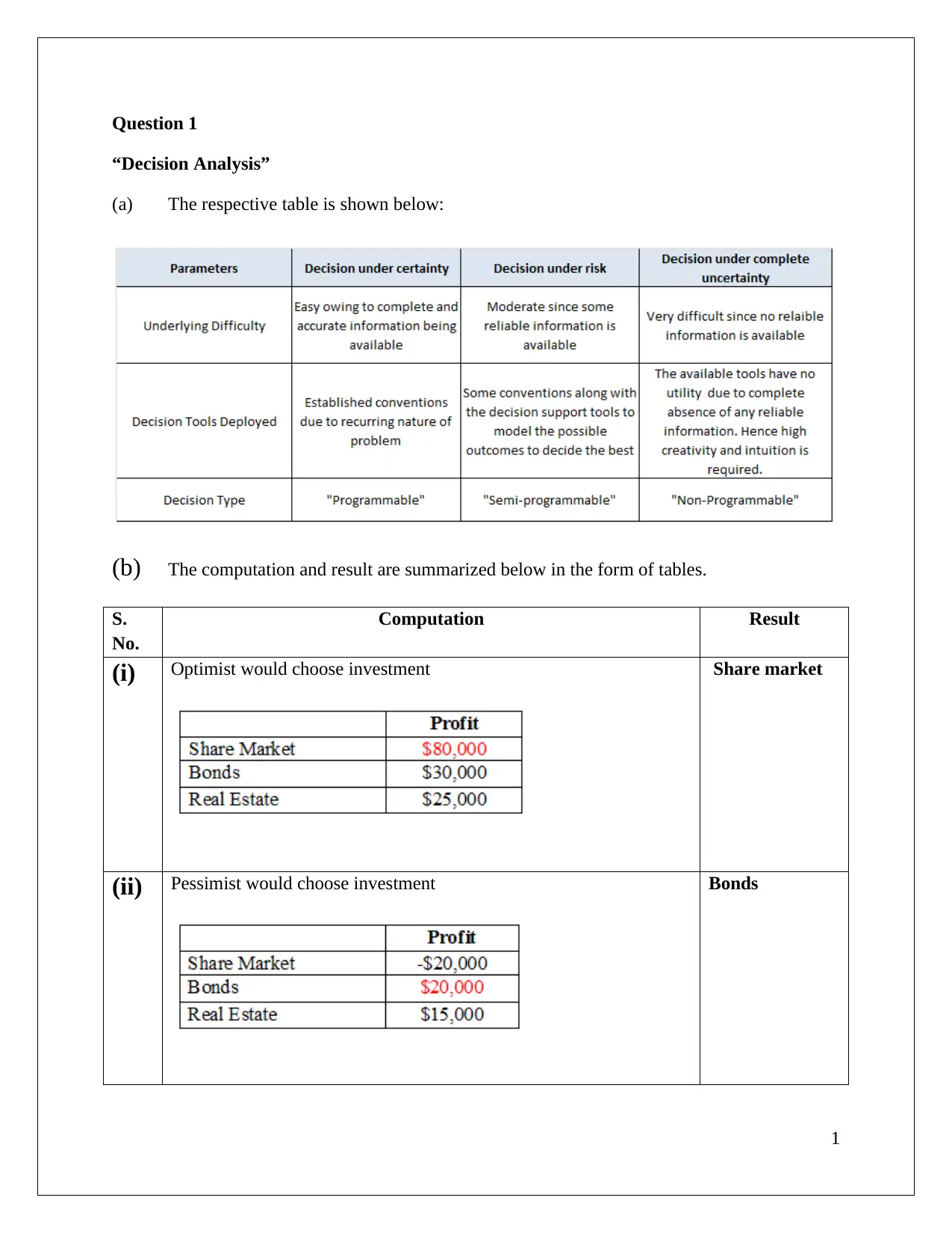
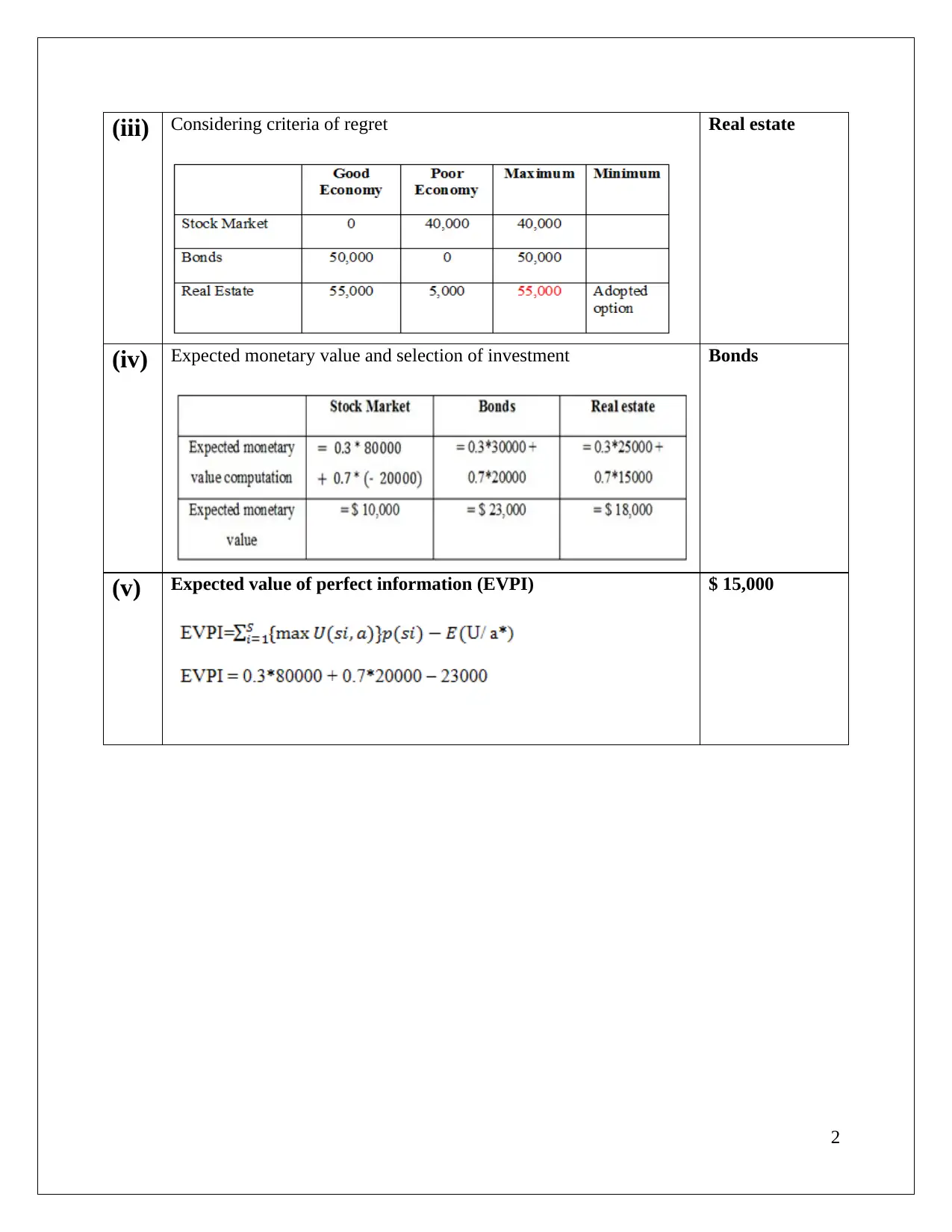
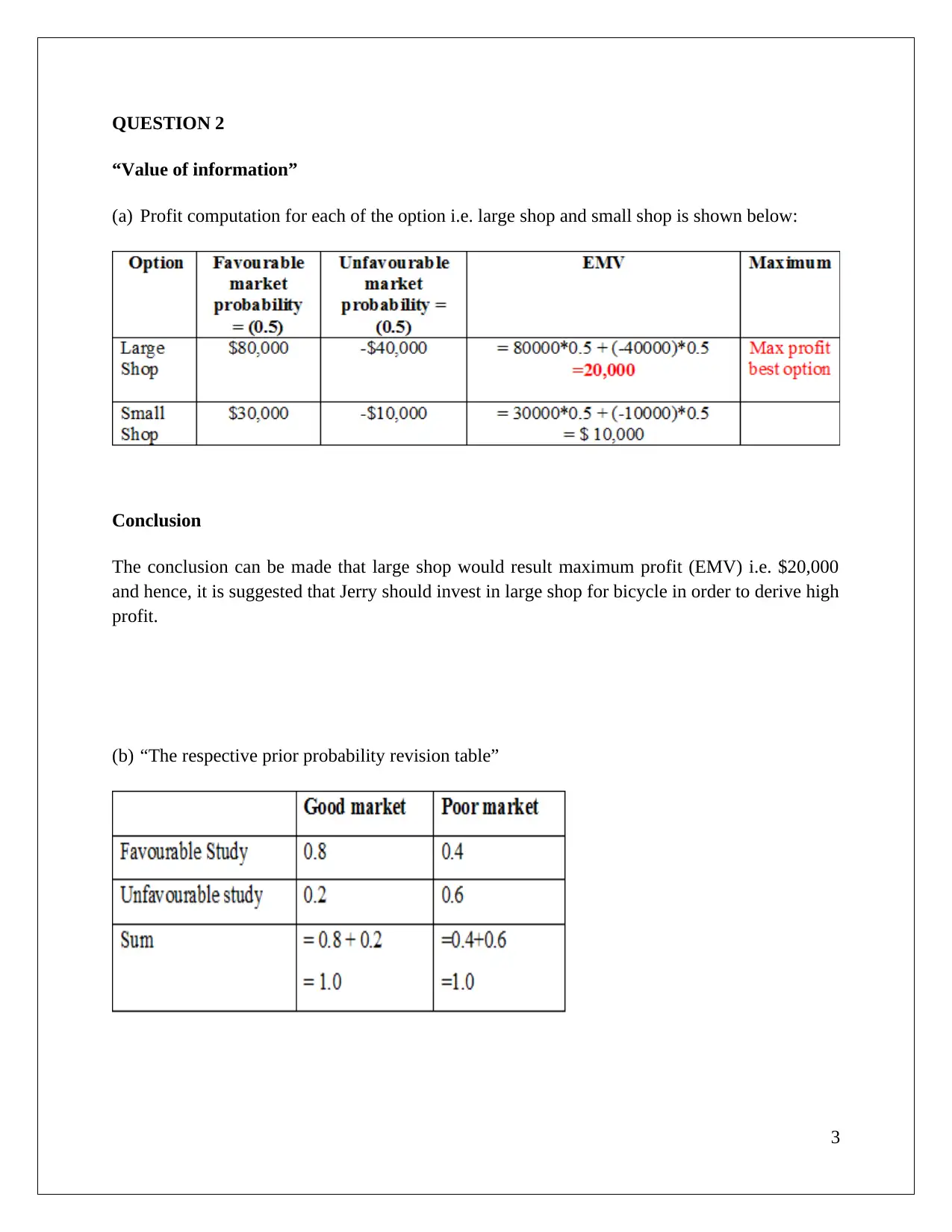
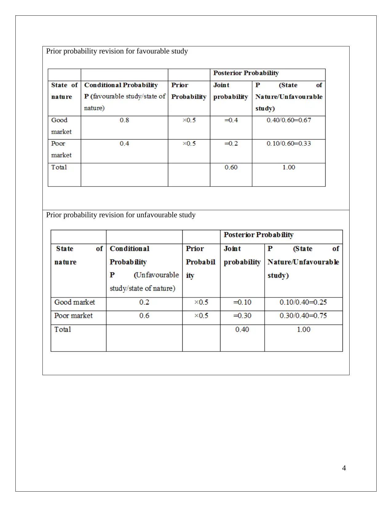
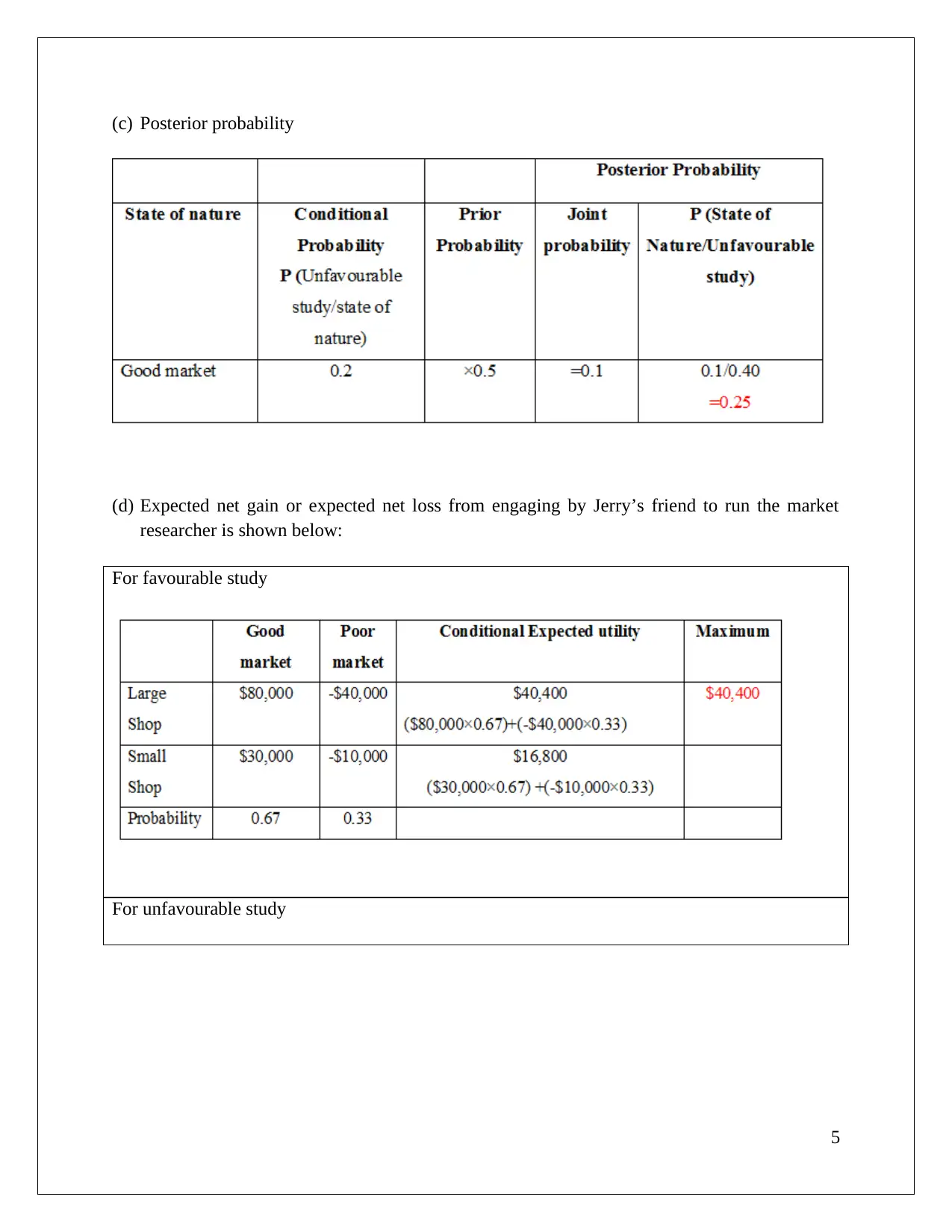
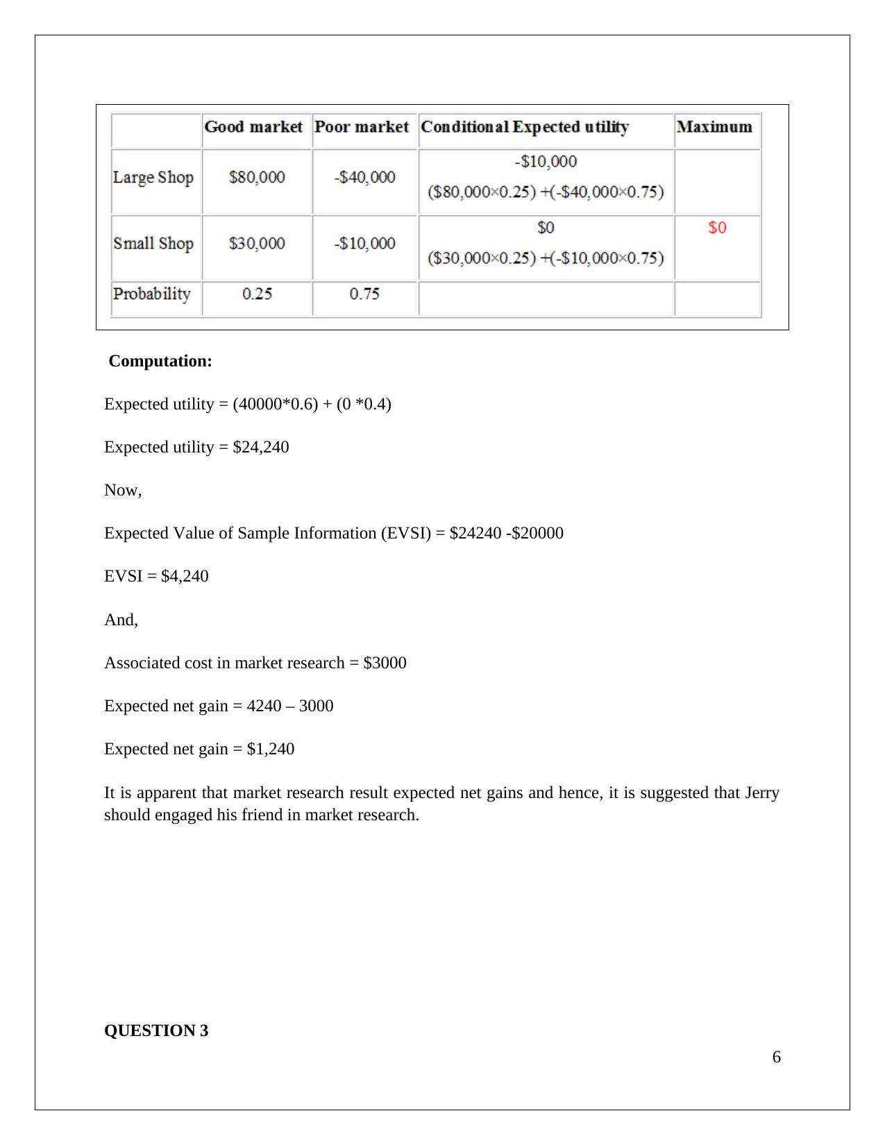
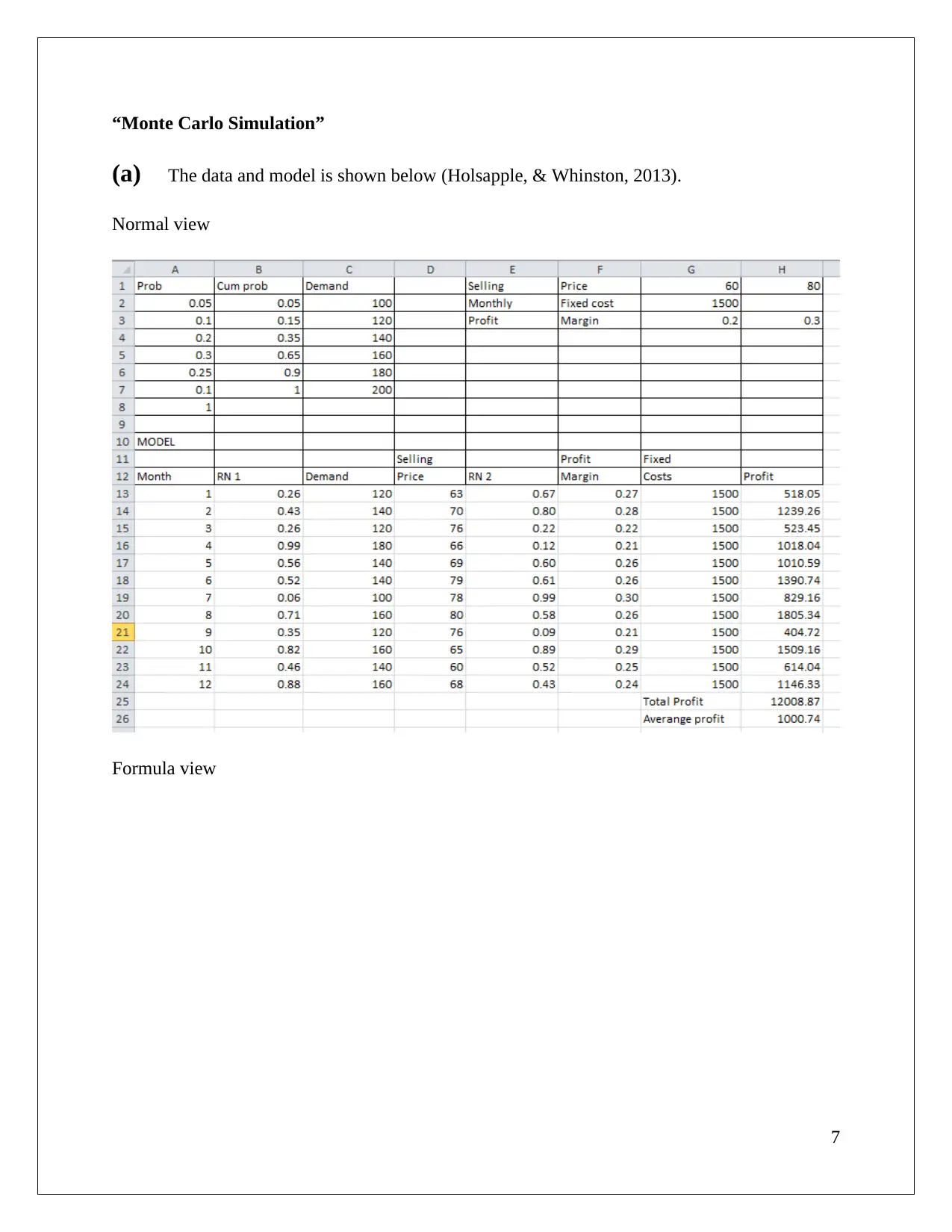
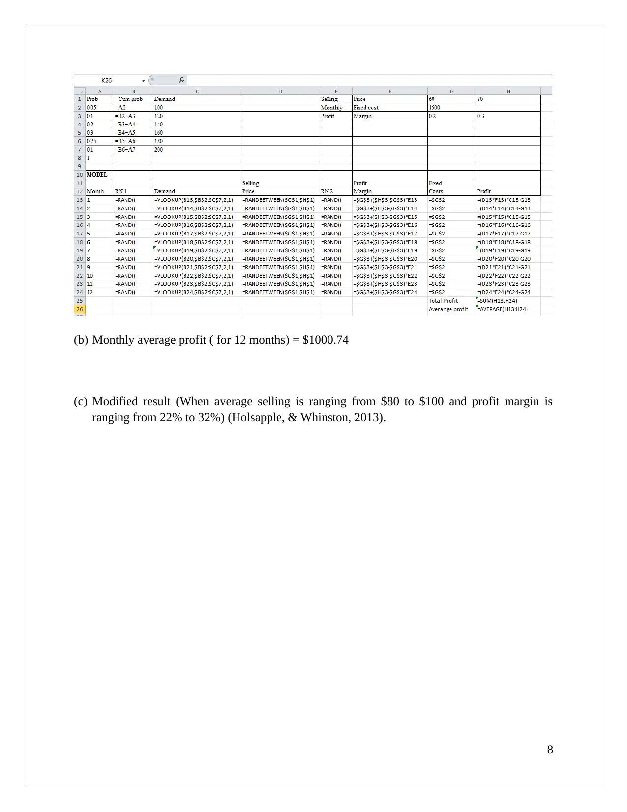
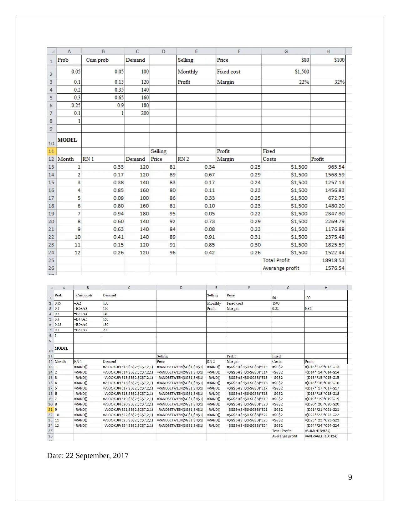
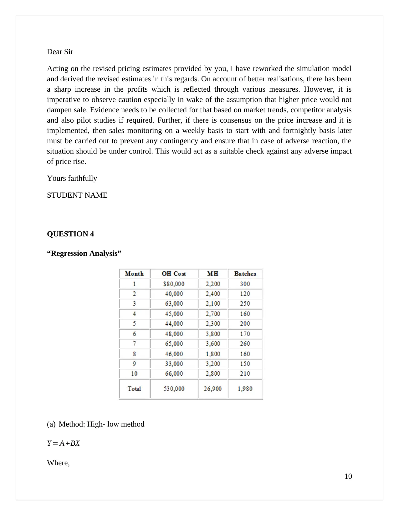
This document presents a comprehensive solution to a Decision Support Tools assignment, addressing various aspects of business decision-making. The assignment covers decision analysis, including the selection of investments based on different criteria and the value of information. It also includ...Read More

DECISION SUPPORT TOOLS
Student id or name
[Pick the date]

Question 1
“Decision Analysis”
(a) The respective table is shown below:
(b) The computation and result are summarized below in the form of tables.
S.
No.
Computation Result
(i) Optimist would choose investment Share market
(ii) Pessimist would choose investment Bonds
1

(iii) Considering criteria of regret Real estate
(iv) Expected monetary value and selection of investment Bonds
(v) Expected value of perfect information (EVPI) $ 15,000
2

QUESTION 2
“Value of information”
(a) Profit computation for each of the option i.e. large shop and small shop is shown below:
Conclusion
The conclusion can be made that large shop would result maximum profit (EMV) i.e. $20,000
and hence, it is suggested that Jerry should invest in large shop for bicycle in order to derive high
profit.
(b) “The respective prior probability revision table”
3

Prior probability revision for favourable study
Prior probability revision for unfavourable study
4

(c) Posterior probability
(d) Expected net gain or expected net loss from engaging by Jerry’s friend to run the market
researcher is shown below:
For favourable study
For unfavourable study
5

Computation:
Expected utility = (40000*0.6) + (0 *0.4)
Expected utility = $24,240
Now,
Expected Value of Sample Information (EVSI) = $24240 -$20000
EVSI = $4,240
And,
Associated cost in market research = $3000
Expected net gain = 4240 – 3000
Expected net gain = $1,240
It is apparent that market research result expected net gains and hence, it is suggested that Jerry
should engaged his friend in market research.
QUESTION 3
6

“Monte Carlo Simulation”
(a) The data and model is shown below (Holsapple, & Whinston, 2013).
Normal view
Formula view
7

(b) Monthly average profit ( for 12 months) = $1000.74
(c) Modified result (When average selling is ranging from $80 to $100 and profit margin is
ranging from 22% to 32%) (Holsapple, & Whinston, 2013).
8

Date: 22 September, 2017
9

Dear Sir
Acting on the revised pricing estimates provided by you, I have reworked the simulation model
and derived the revised estimates in this regards. On account of better realisations, there has been
a sharp increase in the profits which is reflected through various measures. However, it is
imperative to observe caution especially in wake of the assumption that higher price would not
dampen sale. Evidence needs to be collected for that based on market trends, competitor analysis
and also pilot studies if required. Further, if there is consensus on the price increase and it is
implemented, then sales monitoring on a weekly basis to start with and fortnightly basis later
must be carried out to prevent any contingency and ensure that in case of adverse reaction, the
situation should be under control. This would act as a suitable check against any adverse impact
of price rise.
Yours faithfully
STUDENT NAME
QUESTION 4
“Regression Analysis”
(a) Method: High- low method
Y = A +BX
Where,
10

Y =48,000
B=Variable cost per unit= ($48,000-$46,000)/(3800-1800) = $ 1
X =3800 hours
Now,
Y = A +BX
Or
A=Y −BX=48000− ( 1 )∗ ( 3800 ) =$ 44,200
Regression equation through high-low method
Overhead cost (OH) = 44200+ Machine hours
At MH = 3000 hours
Overhead cost (OH) = 44200+ 3000
Overhead cost (OH) = $47,200
(b) Regression
Regression mode 1 – MH is as independent variable
11

Hypothesis testing
Test statistics (t value) = -0.30 and p value = 0.77
Significance level = 5%
Final decision: Fails to reject null hypothesis because p value >> significance level
Conclusion drawn: Slope is not significant.
This is also evident from ANOVA table because in that also, the p value (0.774) is higher than
significance level and thus, the model is not significant (Medhi, 2001).
12

Regression mode 2 – Batches is as independent variable
Hypothesis testing
Test statistics (t value) = 6.28 and p value = 0.00
Significance level = 5%
Final decision: Reject null hypothesis because p value << significance level (Lind, Marchal &
Wathen, 2012)
Conclusion drawn: Slope is statistically significant.
This is also evident from ANOVA table because in that also, the p value (0.0002) is lower than
significance level and thus, the model is statistically significant (Medhi, 2001).
13

Regression mode 3 – Batches and machine hours is as independent variable
Hypothesis testing for machine hours
Test statistics (t value) = -0.27 and p value = 0.79
Significance level = 5%
Final decision: fails to null hypothesis because p value >> significance level
Conclusion drawn: Slope is not significant.
This is also evident from ANOVA table because in that also, the p value (0.001) is lower than
significance level and thus, the model is statistically significant (Medhi, 2001).
14

Hypothesis testing for batches
Test statistics (t value) = 5.87and p value = 0.00
Significance level = 5%
Final decision: reject to null hypothesis because p value << significance level
Conclusion drawn: Slope is statistically significant.
This is also evident from ANOVA table because in that also, the p value (0.00) is lower than
significance level and thus, the model is statistically significant (Hair, 2015).
(c) Ideally R2 is used for highlighting the best model but the presence of different predictor
variables for the models under comparison rules out that possibility. A more accurate
measure would be adjusted R2 since it is not influenced by the underlying independent
variables present. Comparing this value for all the three models, it becomes evident that the
highest value is observed for Model 2 (Using only batches as predictor variable). Thus, this
can be classified as the best regression model from the available choice.
(d) Regression model selected : mode 2
Overhead cost when batches are 150.
15

QUESTION 5
“CVP Analysis”
(a) Unit contribution margin
Product A=sale price of product A−unit variable cost of product A
¿ $ 10−$ 5=$ 5
Product B=sale price of product B−unit variable cost of product B
¿ $ 20−$ 12=$ 8
(b) At break- even cost, no profit would be received because total revenue would be same as
total cost.
Unit break-even for product B = Fixed cost for product B / Unit contribution margin for product
B
= 4000 /8 = 500 units
(c) At break- even cost, no profit would be received because total revenue would be same as
total cost.
Amount at break-even = Fixed cost for product B / Unit contribution margin for product A
= 10*(4000 /5) = $8000
(d) Before tax profit amount is $5000.
Product A to product B ratio = 2: 1
The value of average contribution margin based on above ratio is given below:
¿ {( 1
3 )∗8 }+ {( 2
3 )∗5 }
¿ $ 6
16

Sale volume would be determined as shown below (Taylor & Cihon, 2004).
¿( 5000+ 4000)/6=1500 units
Total number of units of product A = (1500)* (2/3) = 1000 units
Total number of units of product B = (1500)* (1/3) = 500 units
(ii) Post tax profit amount is $21,000.
For the computation, let the amount of pre-tax profit is $k.
The equation can be written as (Taylor & Cihon, 2004)
( 1−0.30 ) x=21000
x=$ 30,000
Hence,
¿( 30000+ 4000)/ 6=5667 units
Total number of units of product A = (5667)* (2/3) = 3778 units
Total number of units of product B = ( 5667)* (1/3) = 1889 units
17

Reference
Hair, J. F., Wolfinbarger, M., Money, A. H., Samouel, P., & Page, M. J. (2015). Essentials of
business research methods (2nd ed.). New York: Routledge.
Holsapple, C. & Whinston, B.A. (2013) Decision Support Systems: Theory and Application (6th
ed.). Sydney: Springer Science & Business Media
Lind, A.D., Marchal, G.W. & Wathen, A.S. (2012). Statistical Techniques in Business and
Economics (15th ed.). New York : McGraw-Hill/Irwin.
Medhi, J. (2001). Statistical Methods: An Introductory Text (4th ed.). Sydney: New Age
International.
Taylor, K. J. & Cihon, C. (2004). Statistical Techniques for Data Analysis (2nd ed.). Melbourne:
CRC Press.
18

19