Decision Support Tools: Investment Analysis and Utility Function
VerifiedAdded on 2023/06/04
|10
|2436
|232
Report
AI Summary
This report provides a detailed analysis of decision support tools, focusing on utility functions and investment strategies. It explains how utility functions are assessed and their role in understanding risk attitudes, elaborating on the standard gamble method for determining utility values. The report then applies these concepts to Alan Barnes' investment decision, comparing investment in the share market versus government bonds under different market conditions using decision matrices, optimistic and pessimistic criteria, regret criterion, expected monetary value, and Expected Value of Perfect Information (EVPI). Furthermore, the report evaluates Jerry's decision to produce electric razors using expected monetary value and revised prior probabilities based on information from a friend. Finally, the report includes a simulation model for Tully Tires, analyzing the sensitivity of net profit to changes in selling price and profit margin, providing recommendations for management based on the simulation results. The analysis incorporates calculations and justifications for each decision-making approach.

Decision Support Tools
Student Name
Institution
Date
Student Name
Institution
Date
Paraphrase This Document
Need a fresh take? Get an instant paraphrase of this document with our AI Paraphraser
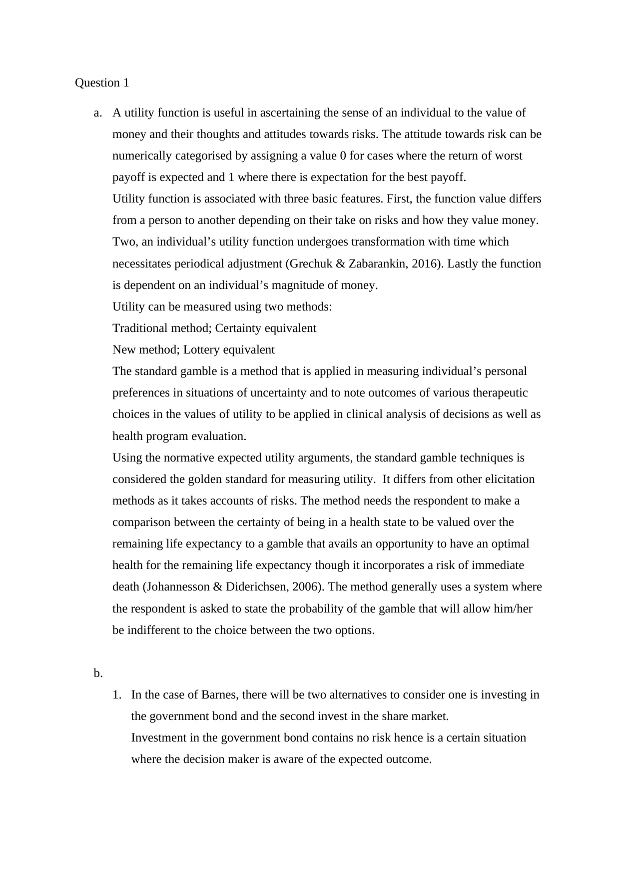
Question 1
a. A utility function is useful in ascertaining the sense of an individual to the value of
money and their thoughts and attitudes towards risks. The attitude towards risk can be
numerically categorised by assigning a value 0 for cases where the return of worst
payoff is expected and 1 where there is expectation for the best payoff.
Utility function is associated with three basic features. First, the function value differs
from a person to another depending on their take on risks and how they value money.
Two, an individual’s utility function undergoes transformation with time which
necessitates periodical adjustment (Grechuk & Zabarankin, 2016). Lastly the function
is dependent on an individual’s magnitude of money.
Utility can be measured using two methods:
Traditional method; Certainty equivalent
New method; Lottery equivalent
The standard gamble is a method that is applied in measuring individual’s personal
preferences in situations of uncertainty and to note outcomes of various therapeutic
choices in the values of utility to be applied in clinical analysis of decisions as well as
health program evaluation.
Using the normative expected utility arguments, the standard gamble techniques is
considered the golden standard for measuring utility. It differs from other elicitation
methods as it takes accounts of risks. The method needs the respondent to make a
comparison between the certainty of being in a health state to be valued over the
remaining life expectancy to a gamble that avails an opportunity to have an optimal
health for the remaining life expectancy though it incorporates a risk of immediate
death (Johannesson & Diderichsen, 2006). The method generally uses a system where
the respondent is asked to state the probability of the gamble that will allow him/her
be indifferent to the choice between the two options.
b.
1. In the case of Barnes, there will be two alternatives to consider one is investing in
the government bond and the second invest in the share market.
Investment in the government bond contains no risk hence is a certain situation
where the decision maker is aware of the expected outcome.
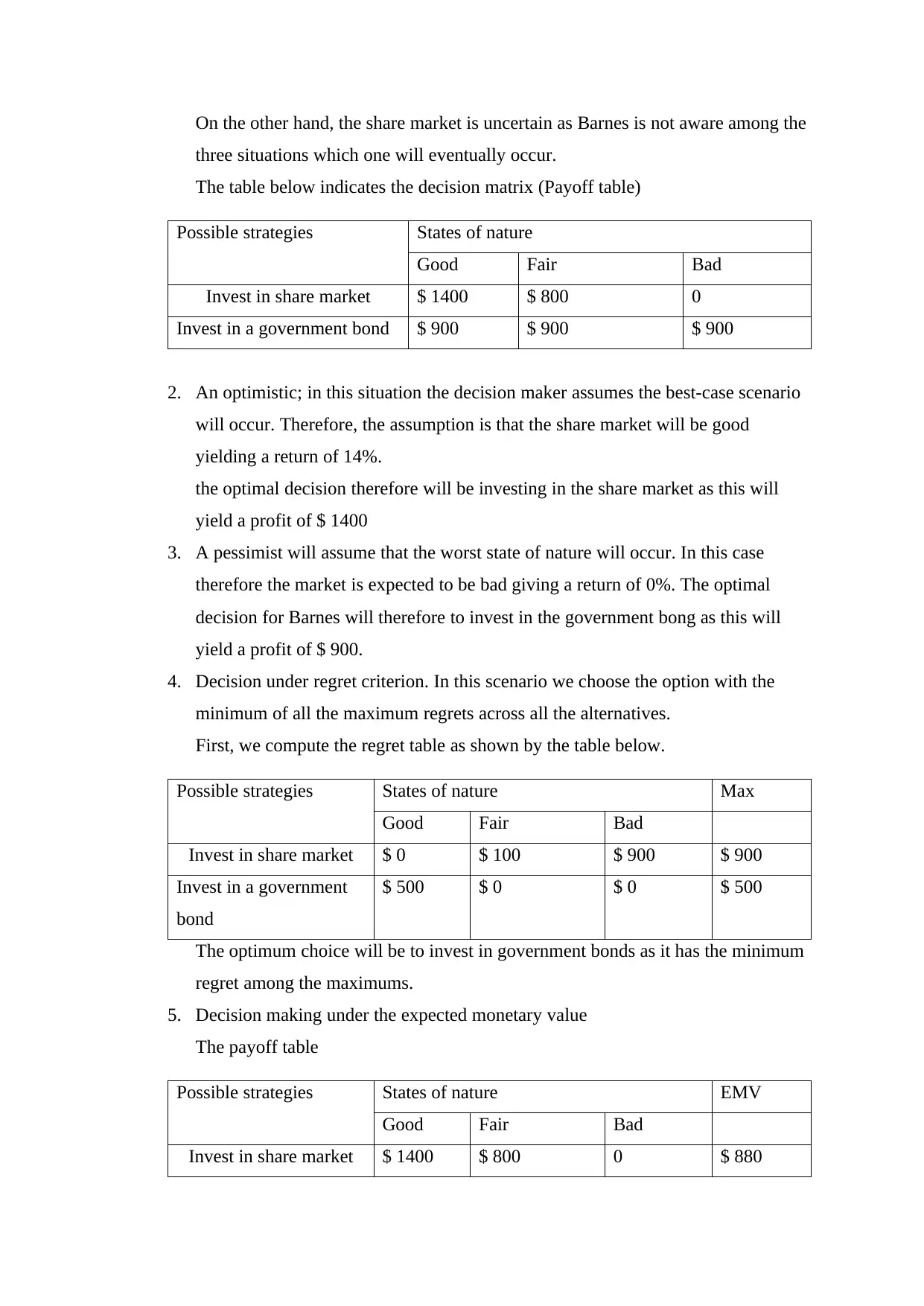
On the other hand, the share market is uncertain as Barnes is not aware among the
three situations which one will eventually occur.
The table below indicates the decision matrix (Payoff table)
Possible strategies States of nature
Good Fair Bad
Invest in share market $ 1400 $ 800 0
Invest in a government bond $ 900 $ 900 $ 900
2. An optimistic; in this situation the decision maker assumes the best-case scenario
will occur. Therefore, the assumption is that the share market will be good
yielding a return of 14%.
the optimal decision therefore will be investing in the share market as this will
yield a profit of $ 1400
3. A pessimist will assume that the worst state of nature will occur. In this case
therefore the market is expected to be bad giving a return of 0%. The optimal
decision for Barnes will therefore to invest in the government bong as this will
yield a profit of $ 900.
4. Decision under regret criterion. In this scenario we choose the option with the
minimum of all the maximum regrets across all the alternatives.
First, we compute the regret table as shown by the table below.
Possible strategies States of nature Max
Good Fair Bad
Invest in share market $ 0 $ 100 $ 900 $ 900
Invest in a government
bond
$ 500 $ 0 $ 0 $ 500
The optimum choice will be to invest in government bonds as it has the minimum
regret among the maximums.
5. Decision making under the expected monetary value
The payoff table
Possible strategies States of nature EMV
Good Fair Bad
Invest in share market $ 1400 $ 800 0 $ 880
You're viewing a preview
Unlock full access by subscribing today!
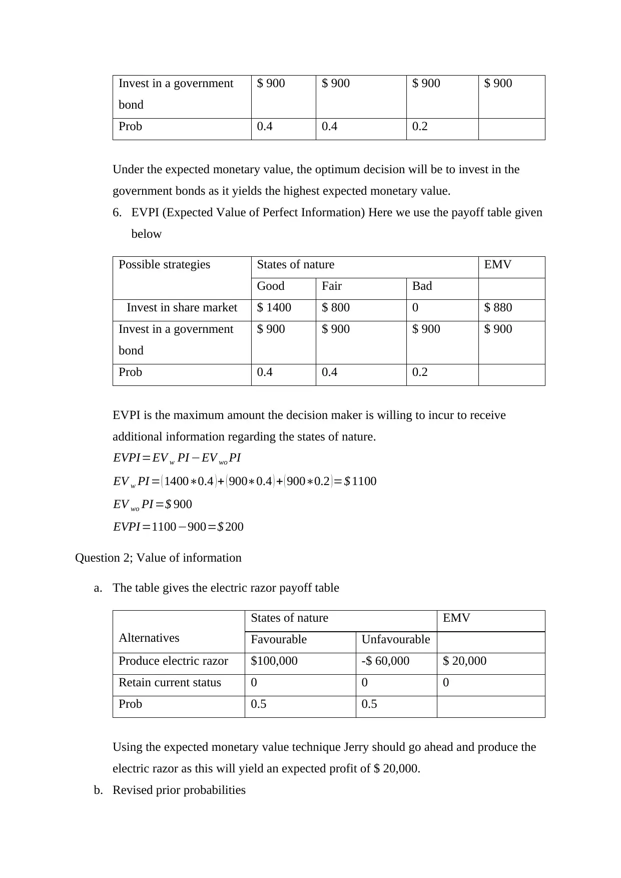
Invest in a government
bond
$ 900 $ 900 $ 900 $ 900
Prob 0.4 0.4 0.2
Under the expected monetary value, the optimum decision will be to invest in the
government bonds as it yields the highest expected monetary value.
6. EVPI (Expected Value of Perfect Information) Here we use the payoff table given
below
Possible strategies States of nature EMV
Good Fair Bad
Invest in share market $ 1400 $ 800 0 $ 880
Invest in a government
bond
$ 900 $ 900 $ 900 $ 900
Prob 0.4 0.4 0.2
EVPI is the maximum amount the decision maker is willing to incur to receive
additional information regarding the states of nature.
EVPI =EV w PI −EV wo PI
EV w PI = ( 1400∗0.4 ) + ( 900∗0.4 ) + ( 900∗0.2 ) =$ 1100
EV wo PI =$ 900
EVPI =1100−900=$ 200
Question 2; Value of information
a. The table gives the electric razor payoff table
Alternatives
States of nature EMV
Favourable Unfavourable
Produce electric razor $100,000 -$ 60,000 $ 20,000
Retain current status 0 0 0
Prob 0.5 0.5
Using the expected monetary value technique Jerry should go ahead and produce the
electric razor as this will yield an expected profit of $ 20,000.
b. Revised prior probabilities
bond
$ 900 $ 900 $ 900 $ 900
Prob 0.4 0.4 0.2
Under the expected monetary value, the optimum decision will be to invest in the
government bonds as it yields the highest expected monetary value.
6. EVPI (Expected Value of Perfect Information) Here we use the payoff table given
below
Possible strategies States of nature EMV
Good Fair Bad
Invest in share market $ 1400 $ 800 0 $ 880
Invest in a government
bond
$ 900 $ 900 $ 900 $ 900
Prob 0.4 0.4 0.2
EVPI is the maximum amount the decision maker is willing to incur to receive
additional information regarding the states of nature.
EVPI =EV w PI −EV wo PI
EV w PI = ( 1400∗0.4 ) + ( 900∗0.4 ) + ( 900∗0.2 ) =$ 1100
EV wo PI =$ 900
EVPI =1100−900=$ 200
Question 2; Value of information
a. The table gives the electric razor payoff table
Alternatives
States of nature EMV
Favourable Unfavourable
Produce electric razor $100,000 -$ 60,000 $ 20,000
Retain current status 0 0 0
Prob 0.5 0.5
Using the expected monetary value technique Jerry should go ahead and produce the
electric razor as this will yield an expected profit of $ 20,000.
b. Revised prior probabilities
Paraphrase This Document
Need a fresh take? Get an instant paraphrase of this document with our AI Paraphraser
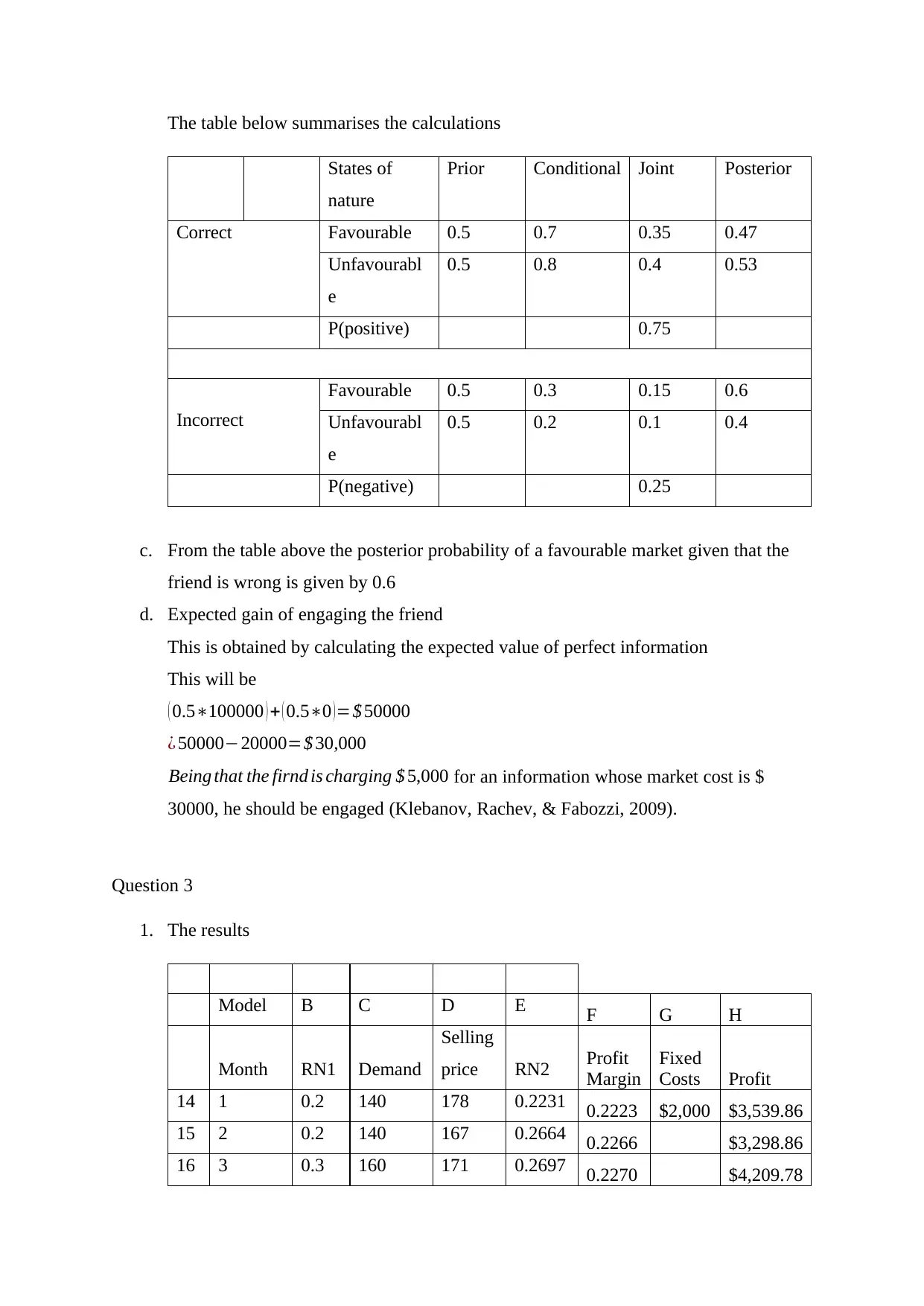
The table below summarises the calculations
States of
nature
Prior Conditional Joint Posterior
Correct Favourable 0.5 0.7 0.35 0.47
Unfavourabl
e
0.5 0.8 0.4 0.53
P(positive) 0.75
Incorrect
Favourable 0.5 0.3 0.15 0.6
Unfavourabl
e
0.5 0.2 0.1 0.4
P(negative) 0.25
c. From the table above the posterior probability of a favourable market given that the
friend is wrong is given by 0.6
d. Expected gain of engaging the friend
This is obtained by calculating the expected value of perfect information
This will be
( 0.5∗100000 ) + ( 0.5∗0 )=$ 50000
¿ 50000−20000=$ 30,000
Being that the firnd is charging $ 5,000 for an information whose market cost is $
30000, he should be engaged (Klebanov, Rachev, & Fabozzi, 2009).
Question 3
1. The results
Model B C D E F G H
Month RN1 Demand
Selling
price RN2 Profit
Margin
Fixed
Costs Profit
14 1 0.2 140 178 0.2231 0.2223 $2,000 $3,539.86
15 2 0.2 140 167 0.2664 0.2266 $3,298.86
16 3 0.3 160 171 0.2697 0.2270 $4,209.78
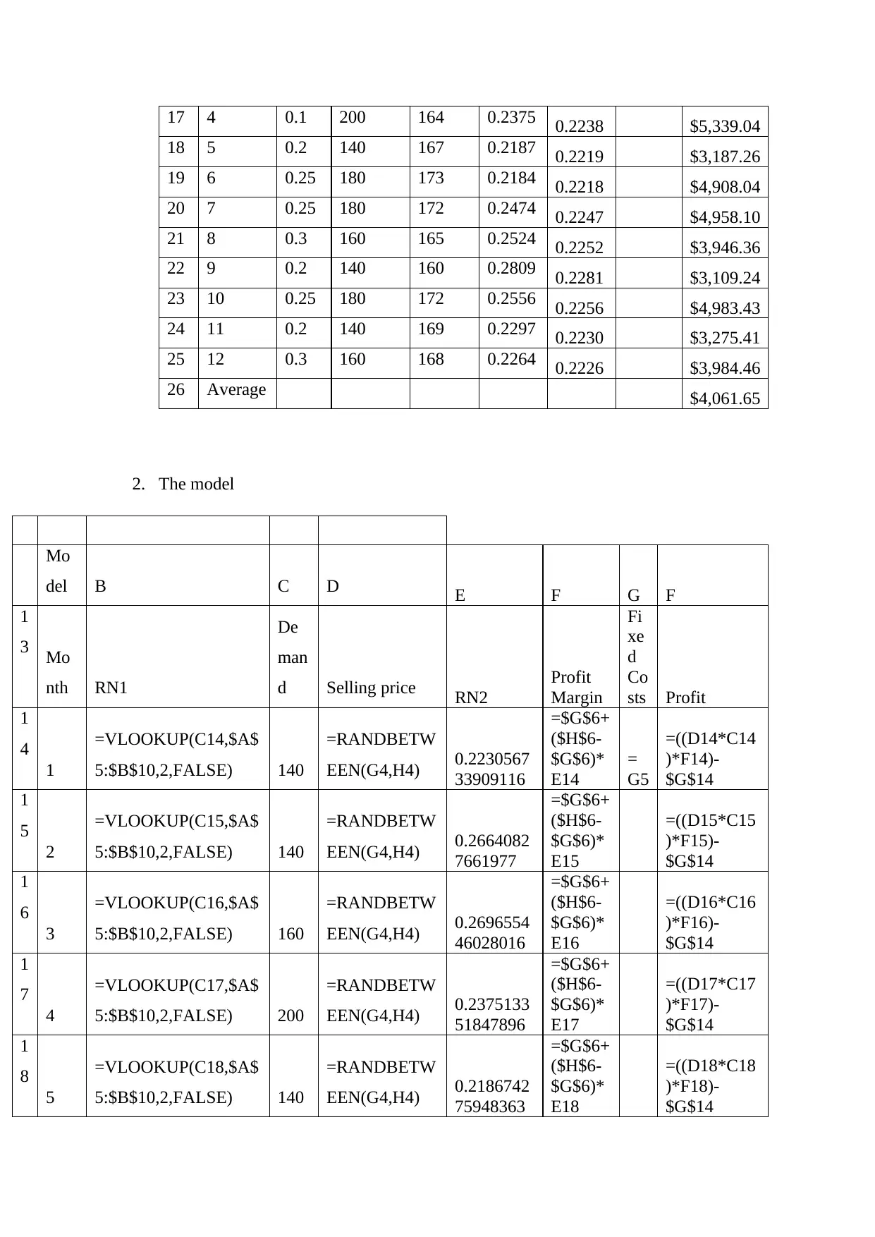
17 4 0.1 200 164 0.2375 0.2238 $5,339.04
18 5 0.2 140 167 0.2187 0.2219 $3,187.26
19 6 0.25 180 173 0.2184 0.2218 $4,908.04
20 7 0.25 180 172 0.2474 0.2247 $4,958.10
21 8 0.3 160 165 0.2524 0.2252 $3,946.36
22 9 0.2 140 160 0.2809 0.2281 $3,109.24
23 10 0.25 180 172 0.2556 0.2256 $4,983.43
24 11 0.2 140 169 0.2297 0.2230 $3,275.41
25 12 0.3 160 168 0.2264 0.2226 $3,984.46
26 Average $4,061.65
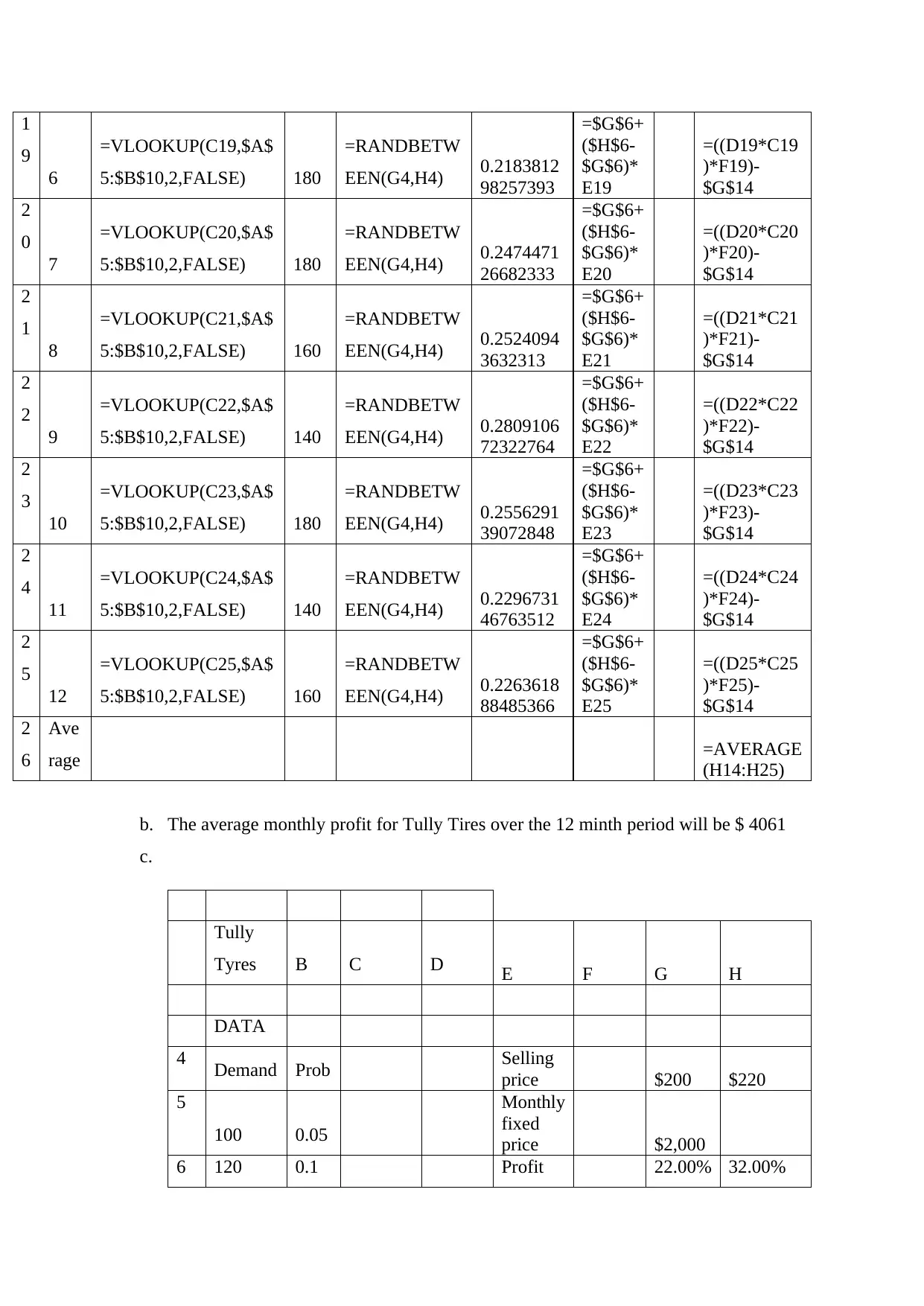
2. The model
Mo
del B C D E F G F
1
3 Mo
nth RN1
De
man
d Selling price RN2
Profit
Margin
Fi
xe
d
Co
sts Profit
1
4
1
=VLOOKUP(C14,$A$
5:$B$10,2,FALSE) 140
=RANDBETW
EEN(G4,H4) 0.2230567
33909116
=$G$6+
($H$6-
$G$6)*
E14
=
G5
=((D14*C14
)*F14)-
$G$14
1
5
2
=VLOOKUP(C15,$A$
5:$B$10,2,FALSE) 140
=RANDBETW
EEN(G4,H4) 0.2664082
7661977
=$G$6+
($H$6-
$G$6)*
E15
=((D15*C15
)*F15)-
$G$14
1
6
3
=VLOOKUP(C16,$A$
5:$B$10,2,FALSE) 160
=RANDBETW
EEN(G4,H4) 0.2696554
46028016
=$G$6+
($H$6-
$G$6)*
E16
=((D16*C16
)*F16)-
$G$14
1
7
4
=VLOOKUP(C17,$A$
5:$B$10,2,FALSE) 200
=RANDBETW
EEN(G4,H4) 0.2375133
51847896
=$G$6+
($H$6-
$G$6)*
E17
=((D17*C17
)*F17)-
$G$14
1
8
5
=VLOOKUP(C18,$A$
5:$B$10,2,FALSE) 140
=RANDBETW
EEN(G4,H4) 0.2186742
75948363
=$G$6+
($H$6-
$G$6)*
E18
=((D18*C18
)*F18)-
$G$14
You're viewing a preview
Unlock full access by subscribing today!
1
9
6
=VLOOKUP(C19,$A$
5:$B$10,2,FALSE) 180
=RANDBETW
EEN(G4,H4) 0.2183812
98257393
=$G$6+
($H$6-
$G$6)*
E19
=((D19*C19
)*F19)-
$G$14
2
0
7
=VLOOKUP(C20,$A$
5:$B$10,2,FALSE) 180
=RANDBETW
EEN(G4,H4) 0.2474471
26682333
=$G$6+
($H$6-
$G$6)*
E20
=((D20*C20
)*F20)-
$G$14
2
1
8
=VLOOKUP(C21,$A$
5:$B$10,2,FALSE) 160
=RANDBETW
EEN(G4,H4) 0.2524094
3632313
=$G$6+
($H$6-
$G$6)*
E21
=((D21*C21
)*F21)-
$G$14
2
2
9
=VLOOKUP(C22,$A$
5:$B$10,2,FALSE) 140
=RANDBETW
EEN(G4,H4) 0.2809106
72322764
=$G$6+
($H$6-
$G$6)*
E22
=((D22*C22
)*F22)-
$G$14
2
3
10
=VLOOKUP(C23,$A$
5:$B$10,2,FALSE) 180
=RANDBETW
EEN(G4,H4) 0.2556291
39072848
=$G$6+
($H$6-
$G$6)*
E23
=((D23*C23
)*F23)-
$G$14
2
4
11
=VLOOKUP(C24,$A$
5:$B$10,2,FALSE) 140
=RANDBETW
EEN(G4,H4) 0.2296731
46763512
=$G$6+
($H$6-
$G$6)*
E24
=((D24*C24
)*F24)-
$G$14
2
5
12
=VLOOKUP(C25,$A$
5:$B$10,2,FALSE) 160
=RANDBETW
EEN(G4,H4) 0.2263618
88485366
=$G$6+
($H$6-
$G$6)*
E25
=((D25*C25
)*F25)-
$G$14
2
6
Ave
rage =AVERAGE
(H14:H25)
b. The average monthly profit for Tully Tires over the 12 minth period will be $ 4061
c.
Tully
Tyres B C D E F G H
DATA
4 Demand Prob Selling
price $200 $220
5
100 0.05
Monthly
fixed
price $2,000
6 120 0.1 Profit 22.00% 32.00%
9
6
=VLOOKUP(C19,$A$
5:$B$10,2,FALSE) 180
=RANDBETW
EEN(G4,H4) 0.2183812
98257393
=$G$6+
($H$6-
$G$6)*
E19
=((D19*C19
)*F19)-
$G$14
2
0
7
=VLOOKUP(C20,$A$
5:$B$10,2,FALSE) 180
=RANDBETW
EEN(G4,H4) 0.2474471
26682333
=$G$6+
($H$6-
$G$6)*
E20
=((D20*C20
)*F20)-
$G$14
2
1
8
=VLOOKUP(C21,$A$
5:$B$10,2,FALSE) 160
=RANDBETW
EEN(G4,H4) 0.2524094
3632313
=$G$6+
($H$6-
$G$6)*
E21
=((D21*C21
)*F21)-
$G$14
2
2
9
=VLOOKUP(C22,$A$
5:$B$10,2,FALSE) 140
=RANDBETW
EEN(G4,H4) 0.2809106
72322764
=$G$6+
($H$6-
$G$6)*
E22
=((D22*C22
)*F22)-
$G$14
2
3
10
=VLOOKUP(C23,$A$
5:$B$10,2,FALSE) 180
=RANDBETW
EEN(G4,H4) 0.2556291
39072848
=$G$6+
($H$6-
$G$6)*
E23
=((D23*C23
)*F23)-
$G$14
2
4
11
=VLOOKUP(C24,$A$
5:$B$10,2,FALSE) 140
=RANDBETW
EEN(G4,H4) 0.2296731
46763512
=$G$6+
($H$6-
$G$6)*
E24
=((D24*C24
)*F24)-
$G$14
2
5
12
=VLOOKUP(C25,$A$
5:$B$10,2,FALSE) 160
=RANDBETW
EEN(G4,H4) 0.2263618
88485366
=$G$6+
($H$6-
$G$6)*
E25
=((D25*C25
)*F25)-
$G$14
2
6
Ave
rage =AVERAGE
(H14:H25)
b. The average monthly profit for Tully Tires over the 12 minth period will be $ 4061
c.
Tully
Tyres B C D E F G H
DATA
4 Demand Prob Selling
price $200 $220
5
100 0.05
Monthly
fixed
price $2,000
6 120 0.1 Profit 22.00% 32.00%
Paraphrase This Document
Need a fresh take? Get an instant paraphrase of this document with our AI Paraphraser
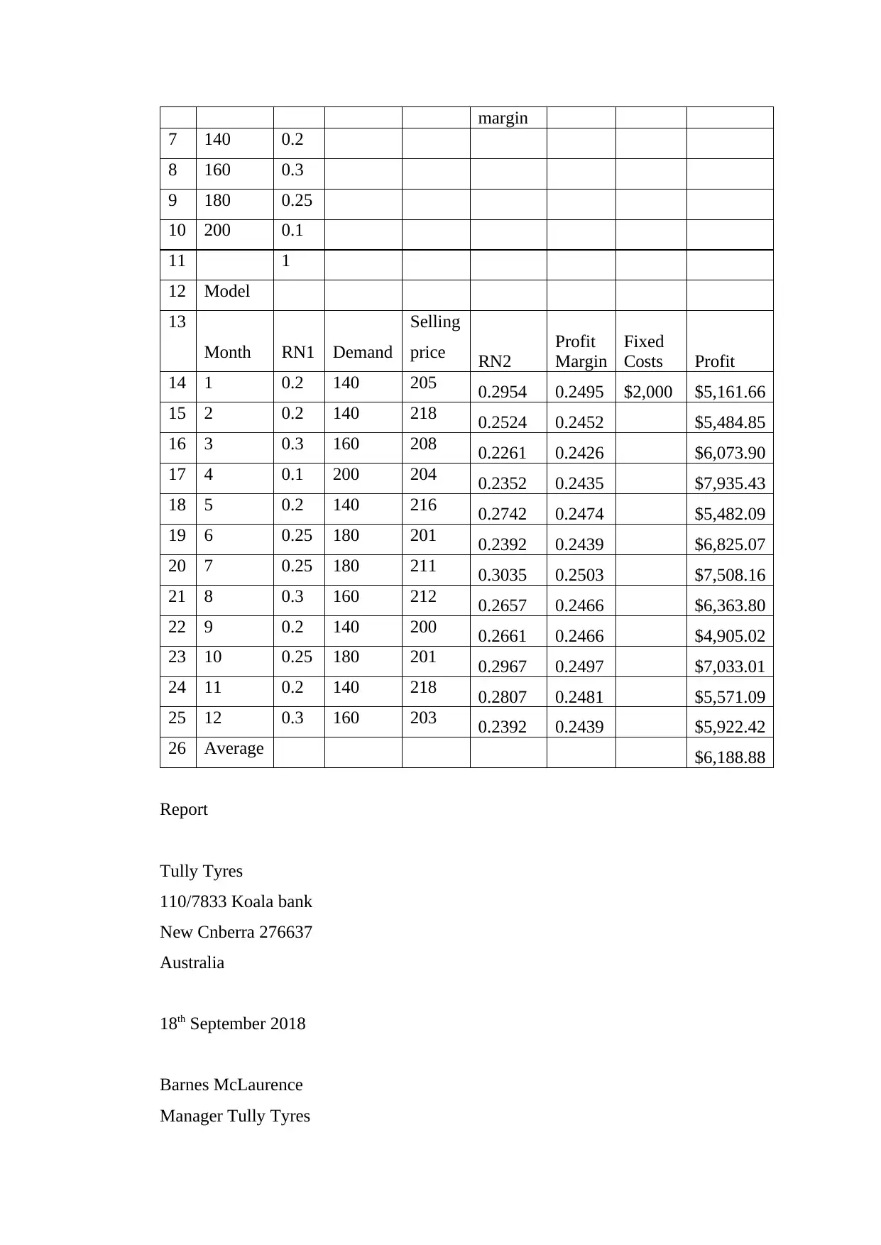
margin
7 140 0.2
8 160 0.3
9 180 0.25
10 200 0.1
11 1
12 Model
13
Month RN1 Demand
Selling
price RN2
Profit
Margin
Fixed
Costs Profit
14 1 0.2 140 205 0.2954 0.2495 $2,000 $5,161.66
15 2 0.2 140 218 0.2524 0.2452 $5,484.85
16 3 0.3 160 208 0.2261 0.2426 $6,073.90
17 4 0.1 200 204 0.2352 0.2435 $7,935.43
18 5 0.2 140 216 0.2742 0.2474 $5,482.09
19 6 0.25 180 201 0.2392 0.2439 $6,825.07
20 7 0.25 180 211 0.3035 0.2503 $7,508.16
21 8 0.3 160 212 0.2657 0.2466 $6,363.80
22 9 0.2 140 200 0.2661 0.2466 $4,905.02
23 10 0.25 180 201 0.2967 0.2497 $7,033.01
24 11 0.2 140 218 0.2807 0.2481 $5,571.09
25 12 0.3 160 203 0.2392 0.2439 $5,922.42
26 Average $6,188.88
Report
Tully Tyres
110/7833 Koala bank
New Cnberra 276637
Australia
18th September 2018
Barnes McLaurence
Manager Tully Tyres
110/7833 Koala bank
New Canberra 276637
Australia
REF:
Dear Mr/Mrs McLaurence,
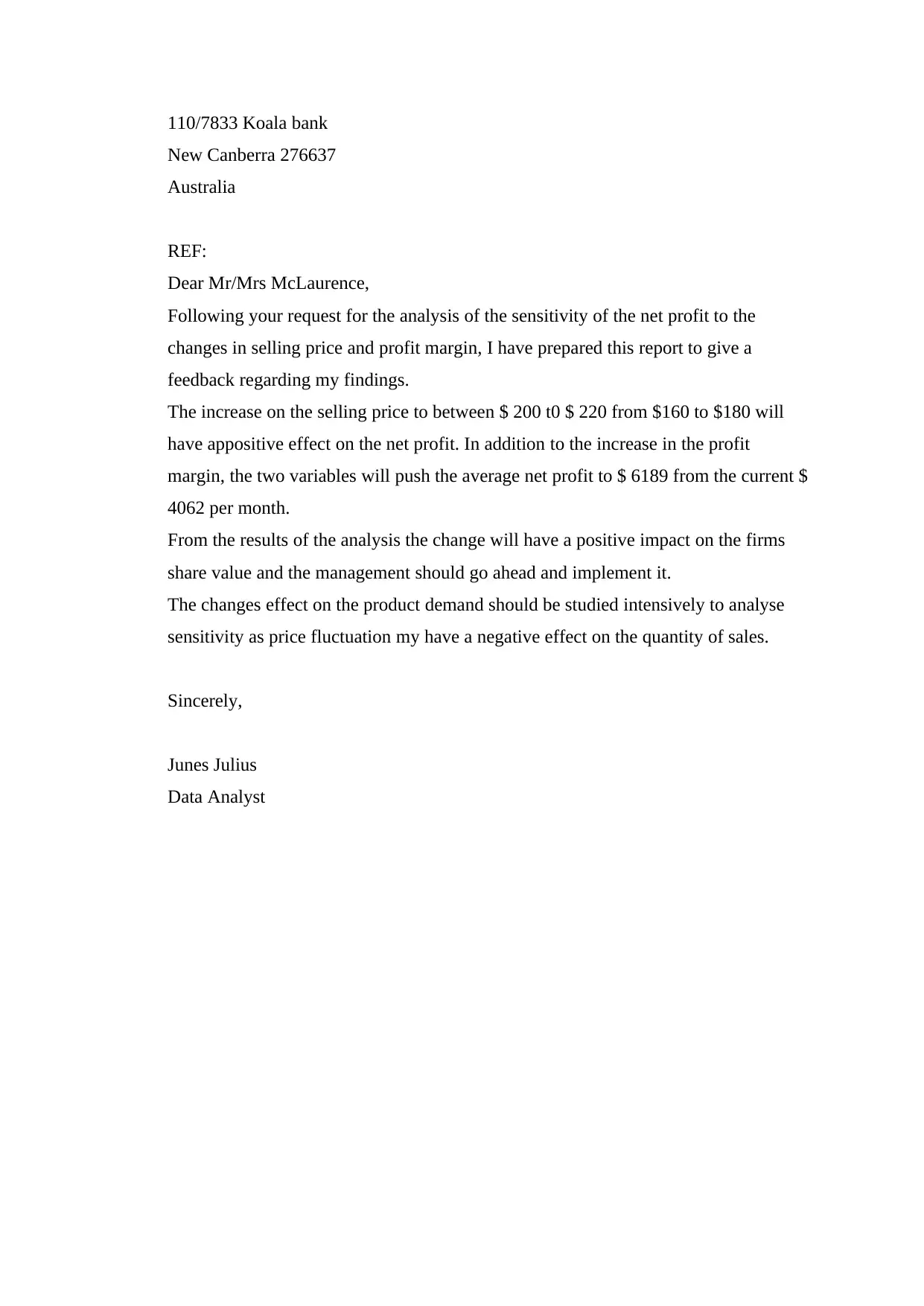
Following your request for the analysis of the sensitivity of the net profit to the
changes in selling price and profit margin, I have prepared this report to give a
feedback regarding my findings.
The increase on the selling price to between $ 200 t0 $ 220 from $160 to $180 will
have appositive effect on the net profit. In addition to the increase in the profit
margin, the two variables will push the average net profit to $ 6189 from the current $
4062 per month.
From the results of the analysis the change will have a positive impact on the firms
share value and the management should go ahead and implement it.
The changes effect on the product demand should be studied intensively to analyse
sensitivity as price fluctuation my have a negative effect on the quantity of sales.
Sincerely,
Junes Julius
Data Analyst
You're viewing a preview
Unlock full access by subscribing today!

References
Grechuk, B., & Zabarankin, M. (2016). Inverse portfolio problem with coherent risk measures .
European Journal of Operational Research, 740-750.
Johannesson, M., & Diderichsen, F. (2006). A comparison of individual and social time-trade-off
values for health states in the general population. Health Policy, 359–370.
Klebanov, L. B., Rachev, S. T., & Fabozzi, F. J. (2009). Non-Robust Models in Statistics. New York: Nova
Scientific Publishers, Inc.
1 out of 10
Related Documents
Your All-in-One AI-Powered Toolkit for Academic Success.
+13062052269
info@desklib.com
Available 24*7 on WhatsApp / Email
![[object Object]](/_next/static/media/star-bottom.7253800d.svg)
Unlock your academic potential
© 2024 | Zucol Services PVT LTD | All rights reserved.


