Decision Support Tools for Desklib Online Library

This article discusses decision support tools and their applications in making effective decisions. It includes solved assignments, essays, and dissertations on decision support tools. The article covers topics such as utility function, investment decisions, market analysis, simulation, regression analysis, and break-even analysis. The content is relevant for students pursuing courses in business, management, and economics.

Running Head: DECISION SUPPORT TOOLS
Decision Support Tools
Name of the Student
Name of the University
Author Note

1DECISION SUPPORT TOOLS
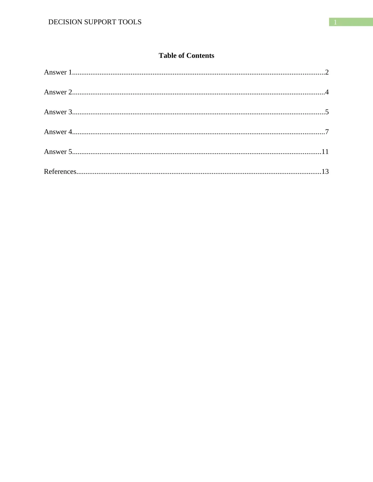
Table of Contents
Answer 1..........................................................................................................................................2
Answer 2..........................................................................................................................................4
Answer 3..........................................................................................................................................5
Answer 4..........................................................................................................................................7
Answer 5........................................................................................................................................11
References......................................................................................................................................13

2DECISION SUPPORT TOOLS
Answer 1
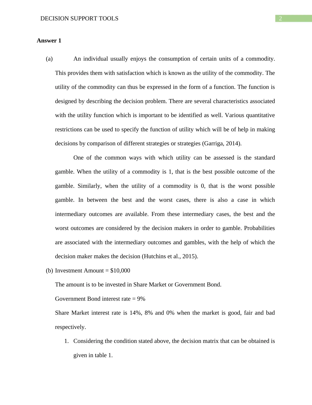
(a) An individual usually enjoys the consumption of certain units of a commodity.
This provides them with satisfaction which is known as the utility of the commodity. The
utility of the commodity can thus be expressed in the form of a function. The function is
designed by describing the decision problem. There are several characteristics associated
with the utility function which is important to be identified as well. Various quantitative
restrictions can be used to specify the function of utility which will be of help in making
decisions by comparison of different strategies or strategies (Garriga, 2014).
One of the common ways with which utility can be assessed is the standard
gamble. When the utility of a commodity is 1, that is the best possible outcome of the
gamble. Similarly, when the utility of a commodity is 0, that is the worst possible
gamble. In between the best and the worst cases, there is also a case in which
intermediary outcomes are available. From these intermediary cases, the best and the
worst outcomes are considered by the decision makers in order to gamble. Probabilities
are associated with the intermediary outcomes and gambles, with the help of which the
decision maker makes the decision (Hutchins et al., 2015).
(b) Investment Amount = $10,000
The amount is to be invested in Share Market or Government Bond.
Government Bond interest rate = 9%
Share Market interest rate is 14%, 8% and 0% when the market is good, fair and bad
respectively.
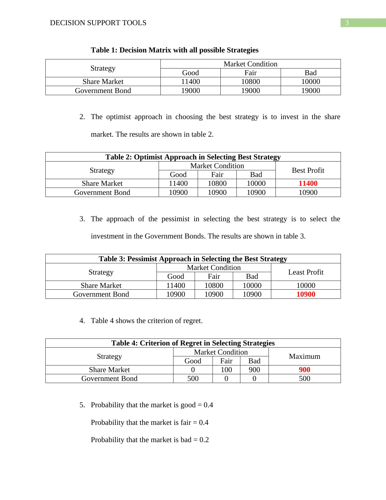
1. Considering the condition stated above, the decision matrix that can be obtained is
given in table 1.

3DECISION SUPPORT TOOLS
Table 1: Decision Matrix with all possible Strategies
Strategy Market Condition
Good Fair Bad
Share Market 11400 10800 10000
Government Bond 19000 19000 19000
2. The optimist approach in choosing the best strategy is to invest in the share
market. The results are shown in table 2.
Table 2: Optimist Approach in Selecting Best Strategy
Strategy Market Condition Best Profit
Good Fair Bad
Share Market 11400 10800 10000 11400
Government Bond 10900 10900 10900 10900
3. The approach of the pessimist in selecting the best strategy is to select the
investment in the Government Bonds. The results are shown in table 3.
Table 3: Pessimist Approach in Selecting the Best Strategy
Strategy Market Condition Least Profit
Good Fair Bad
Share Market 11400 10800 10000 10000
Government Bond 10900 10900 10900 10900
4. Table 4 shows the criterion of regret.
Table 4: Criterion of Regret in Selecting Strategies
Strategy Market Condition Maximum
Good Fair Bad
Share Market 0 100 900 900
Government Bond 500 0 0 500
5. Probability that the market is good = 0.4
Probability that the market is fair = 0.4
Probability that the market is bad = 0.2

4DECISION SUPPORT TOOLS
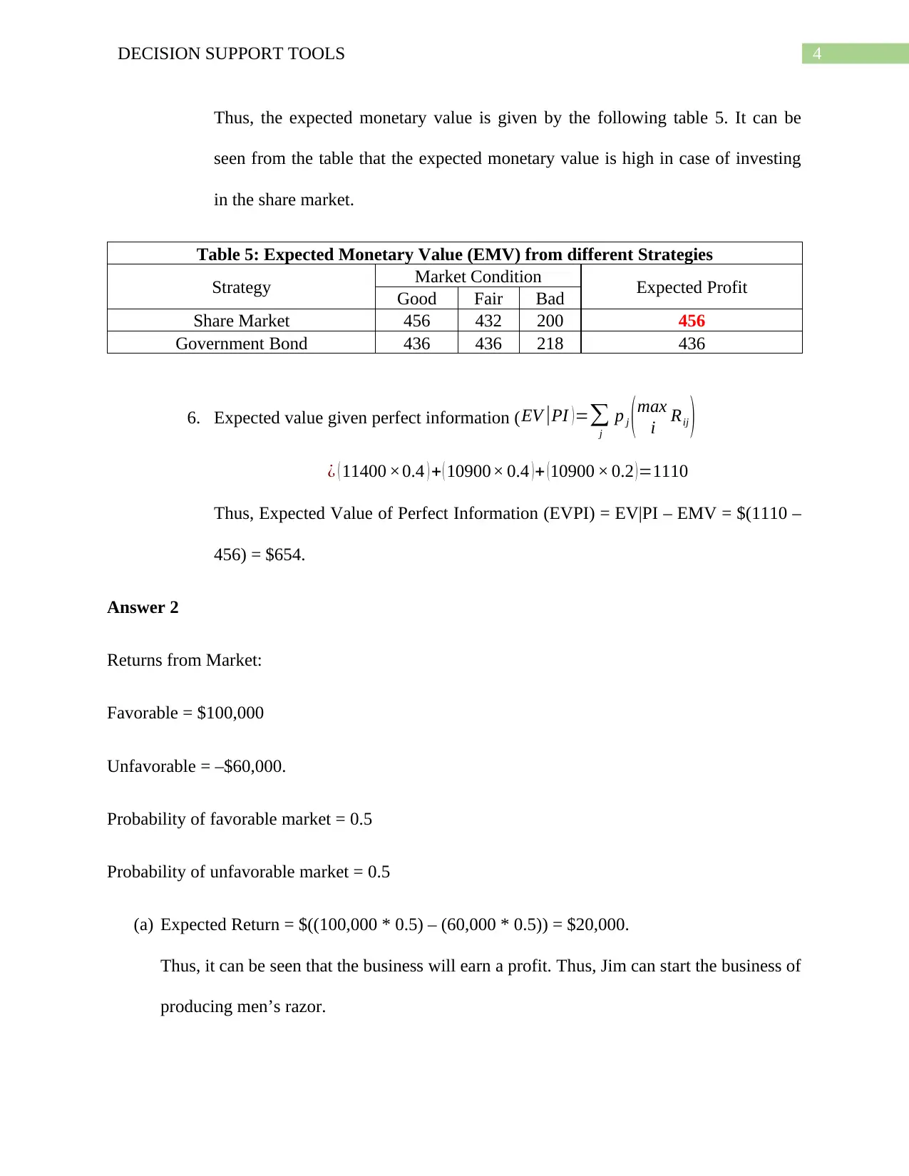
Thus, the expected monetary value is given by the following table 5. It can be
seen from the table that the expected monetary value is high in case of investing
in the share market.
Table 5: Expected Monetary Value (EMV) from different Strategies
Strategy Market Condition Expected Profit
Good Fair Bad
Share Market 456 432 200 456
Government Bond 436 436 218 436
6. Expected value given perfect information ( EV |PI ) =∑
j
p j ( max
i Rij )
¿ ( 11400 ×0.4 ) + ( 10900× 0.4 )+ (10900 × 0.2 )=1110
Thus, Expected Value of Perfect Information (EVPI) = EV|PI – EMV = $(1110 –
456) = $654.
Answer 2
Returns from Market:
Favorable = $100,000
Unfavorable = –$60,000.
Probability of favorable market = 0.5
Probability of unfavorable market = 0.5
(a) Expected Return = $((100,000 * 0.5) – (60,000 * 0.5)) = $20,000.
Thus, it can be seen that the business will earn a profit. Thus, Jim can start the business of
producing men’s razor.

5DECISION SUPPORT TOOLS
(b) Probability of favorable market depending on the track record of his friend = (0.5 * 0.7) +
(0.5 * 0.3) = 0.5. Therefore, the probability of unfavorable market = (1 – 0.5) = 0.5.
(c) The required posterior probability = (0.3 * 0.5) = 0.15.
(d) Expected net gain / loss = $((100,000 * 0.5) + (– 60,000 * 0.5)) – $5,000 = $15,000.
Engagement of friend has decreased the expected profit margin but there is still
profit from the business. Engaging the friend is thus a better choice as his engagement
will provide the market conditions more accurately.
Answer 3
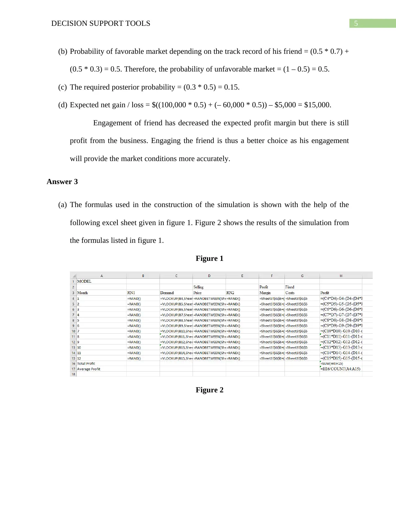
(a) The formulas used in the construction of the simulation is shown with the help of the
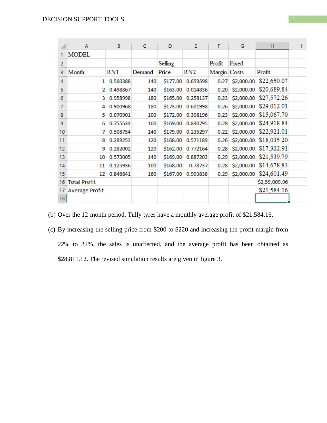
following excel sheet given in figure 1. Figure 2 shows the results of the simulation from
the formulas listed in figure 1.
Figure 1
Figure 2

6DECISION SUPPORT TOOLS
(b) Over the 12-month period, Tully tyres have a monthly average profit of $21,584.16.
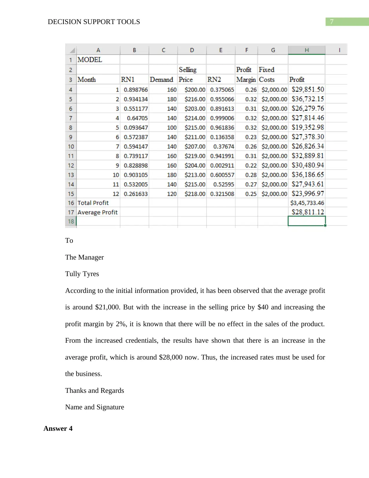
(c) By increasing the selling price from $200 to $220 and increasing the profit margin from
22% to 32%, the sales is unaffected, and the average profit has been obtained as
$28,811.12. The revised simulation results are given in figure 3.

7DECISION SUPPORT TOOLS
To
The Manager
Tully Tyres
According to the initial information provided, it has been observed that the average profit
is around $21,000. But with the increase in the selling price by $40 and increasing the
profit margin by 2%, it is known that there will be no effect in the sales of the product.
From the increased credentials, the results have shown that there is an increase in the
average profit, which is around $28,000 now. Thus, the increased rates must be used for
the business.
Thanks and Regards
Name and Signature
Answer 4

8DECISION SUPPORT TOOLS
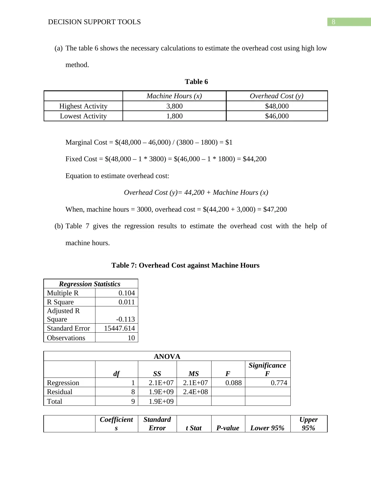
(a) The table 6 shows the necessary calculations to estimate the overhead cost using high low
method.
Table 6
Machine Hours (x) Overhead Cost (y)
Highest Activity 3,800 $48,000
Lowest Activity 1,800 $46,000
Marginal Cost = $(48,000 – 46,000) / (3800 – 1800) = $1
Fixed Cost = $(48,000 – 1 * 3800) = $(46,000 – 1 * 1800) = $44,200
Equation to estimate overhead cost:
Overhead Cost (y)= 44,200 + Machine Hours (x)
When, machine hours = 3000, overhead cost = $(44,200 + 3,000) = $47,200
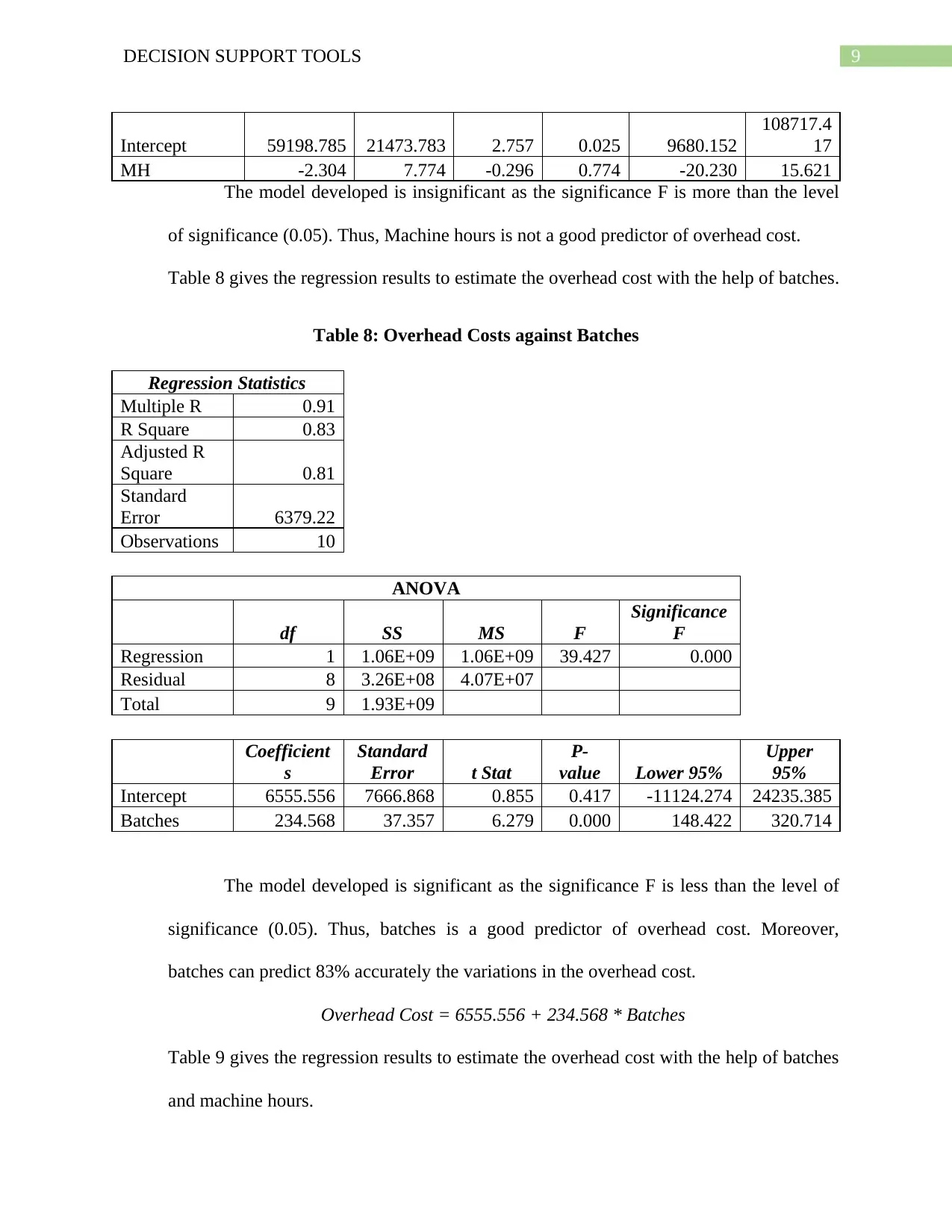
(b) Table 7 gives the regression results to estimate the overhead cost with the help of
machine hours.
Table 7: Overhead Cost against Machine Hours
Regression Statistics
Multiple R 0.104
R Square 0.011
Adjusted R
Square -0.113
Standard Error 15447.614
Observations 10
ANOVA
df SS MS F
Significance
F
Regression 1 2.1E+07 2.1E+07 0.088 0.774
Residual 8 1.9E+09 2.4E+08
Total 9 1.9E+09
Coefficient
s
Standard
Error t Stat P-value Lower 95%
Upper
95%

9DECISION SUPPORT TOOLS
Intercept 59198.785 21473.783 2.757 0.025 9680.152
108717.4
17
MH -2.304 7.774 -0.296 0.774 -20.230 15.621
The model developed is insignificant as the significance F is more than the level
of significance (0.05). Thus, Machine hours is not a good predictor of overhead cost.
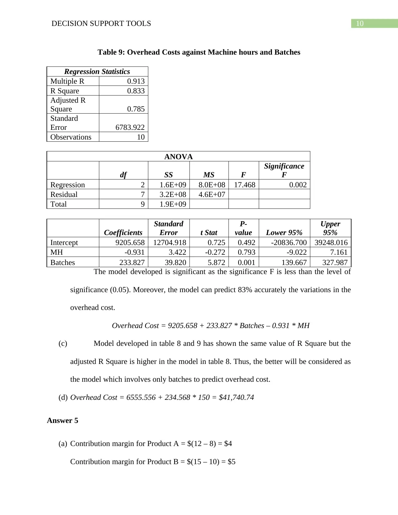
Table 8 gives the regression results to estimate the overhead cost with the help of batches.
Table 8: Overhead Costs against Batches
Regression Statistics
Multiple R 0.91
R Square 0.83
Adjusted R
Square 0.81
Standard
Error 6379.22
Observations 10
ANOVA
df SS MS F
Significance
F
Regression 1 1.06E+09 1.06E+09 39.427 0.000
Residual 8 3.26E+08 4.07E+07
Total 9 1.93E+09
Coefficient
s
Standard
Error t Stat
P-
value Lower 95%
Upper
95%
Intercept 6555.556 7666.868 0.855 0.417 -11124.274 24235.385
Batches 234.568 37.357 6.279 0.000 148.422 320.714
The model developed is significant as the significance F is less than the level of
significance (0.05). Thus, batches is a good predictor of overhead cost. Moreover,
batches can predict 83% accurately the variations in the overhead cost.
Overhead Cost = 6555.556 + 234.568 * Batches
Table 9 gives the regression results to estimate the overhead cost with the help of batches
and machine hours.

10DECISION SUPPORT TOOLS
Table 9: Overhead Costs against Machine hours and Batches
Regression Statistics
Multiple R 0.913
R Square 0.833
Adjusted R
Square 0.785
Standard
Error 6783.922
Observations 10
ANOVA
df SS MS F
Significance
F
Regression 2 1.6E+09 8.0E+08 17.468 0.002
Residual 7 3.2E+08 4.6E+07
Total 9 1.9E+09
Coefficients
Standard
Error t Stat
P-
value Lower 95%
Upper
95%
Intercept 9205.658 12704.918 0.725 0.492 -20836.700 39248.016
MH -0.931 3.422 -0.272 0.793 -9.022 7.161
Batches 233.827 39.820 5.872 0.001 139.667 327.987
The model developed is significant as the significance F is less than the level of
significance (0.05). Moreover, the model can predict 83% accurately the variations in the
overhead cost.
Overhead Cost = 9205.658 + 233.827 * Batches – 0.931 * MH
(c) Model developed in table 8 and 9 has shown the same value of R Square but the
adjusted R Square is higher in the model in table 8. Thus, the better will be considered as
the model which involves only batches to predict overhead cost.
(d) Overhead Cost = 6555.556 + 234.568 * 150 = $41,740.74
Answer 5
(a) Contribution margin for Product A = $(12 – 8) = $4
Contribution margin for Product B = $(15 – 10) = $5

11DECISION SUPPORT TOOLS
(b) For Product B, break even = (5000 / 5) = 1000 units
(c) For Product A, break even = (5000 / 4) = 1250 units
(d) Ratio of manufacture of A and B is 3:1.
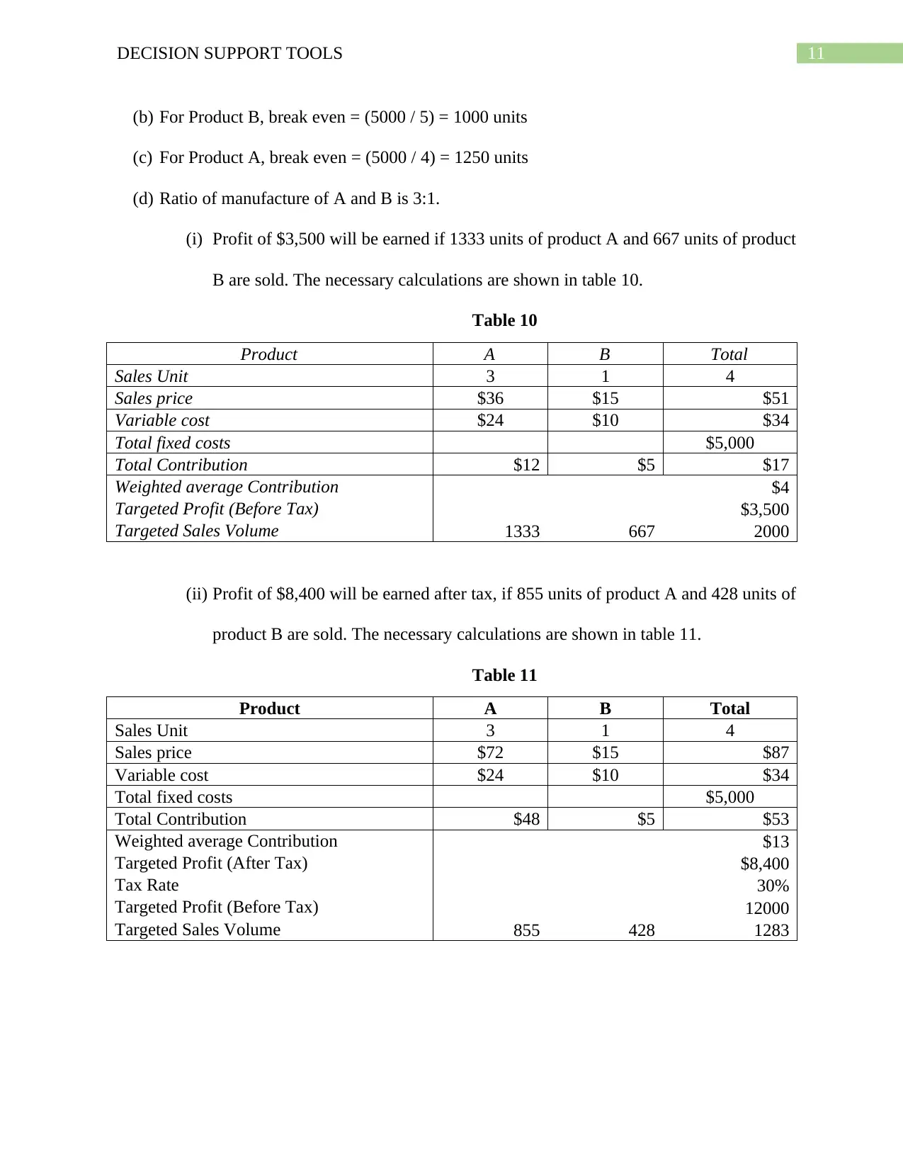
(i) Profit of $3,500 will be earned if 1333 units of product A and 667 units of product
B are sold. The necessary calculations are shown in table 10.
Table 10
Product A B Total
Sales Unit 3 1 4
Sales price $36 $15 $51
Variable cost $24 $10 $34
Total fixed costs $5,000
Total Contribution $12 $5 $17
Weighted average Contribution $4
Targeted Profit (Before Tax) $3,500
Targeted Sales Volume 1333 667 2000
(ii) Profit of $8,400 will be earned after tax, if 855 units of product A and 428 units of
product B are sold. The necessary calculations are shown in table 11.
Table 11
Product A B Total
Sales Unit 3 1 4
Sales price $72 $15 $87
Variable cost $24 $10 $34
Total fixed costs $5,000
Total Contribution $48 $5 $53
Weighted average Contribution $13
Targeted Profit (After Tax) $8,400
Tax Rate 30%
Targeted Profit (Before Tax) 12000
Targeted Sales Volume 855 428 1283

12DECISION SUPPORT TOOLS
References
Garriga, E. (2014). Beyond stakeholder utility function: Stakeholder capability in the value
creation process. Journal of Business Ethics, 120(4), 489-507.
Hutchins, R., Viera, A. J., Sheridan, S. L., & Pignone, M. P. (2015). Quantifying the utility of
taking pills for cardiovascular prevention. Circulation: Cardiovascular Quality and
Outcomes, 8(2), 155-163.