Kingston University CE6106 Project Management Assignment Report

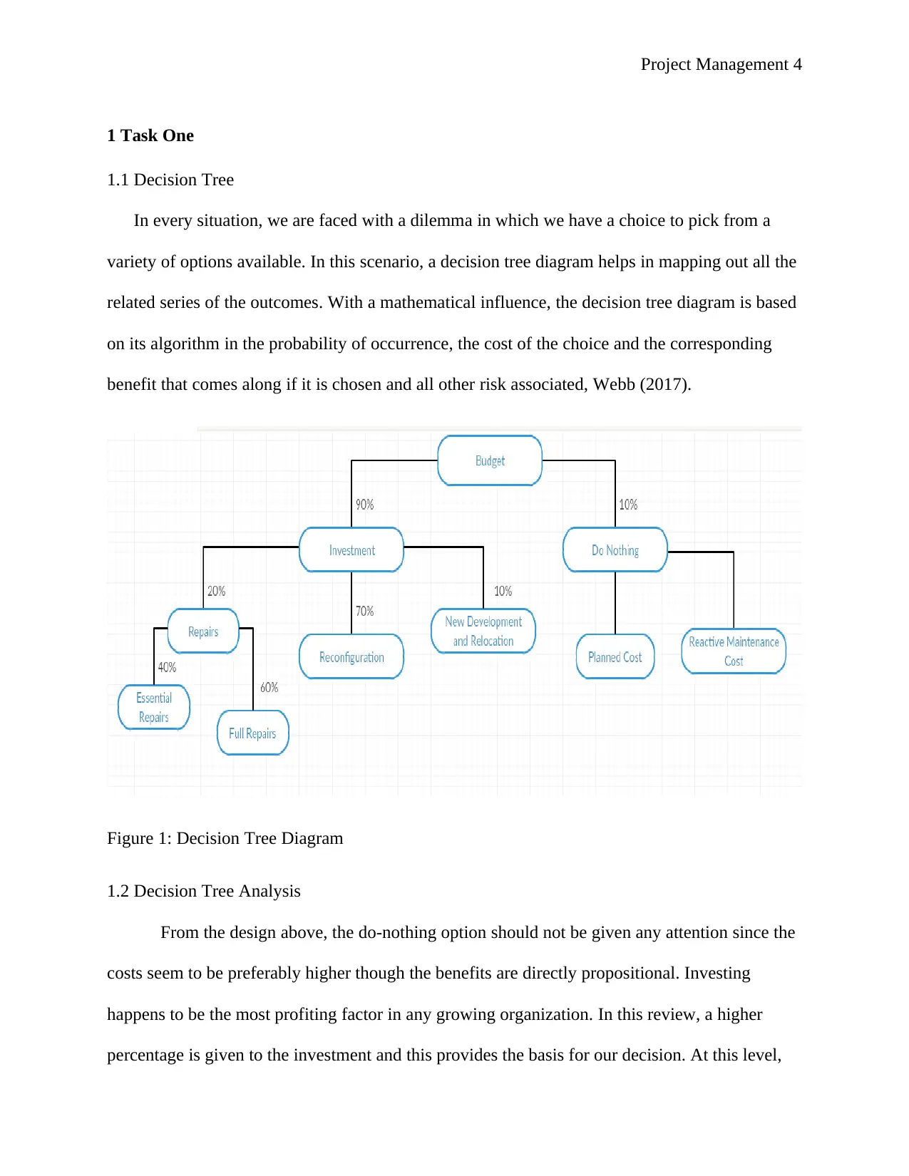
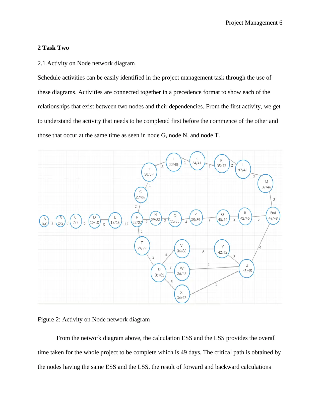
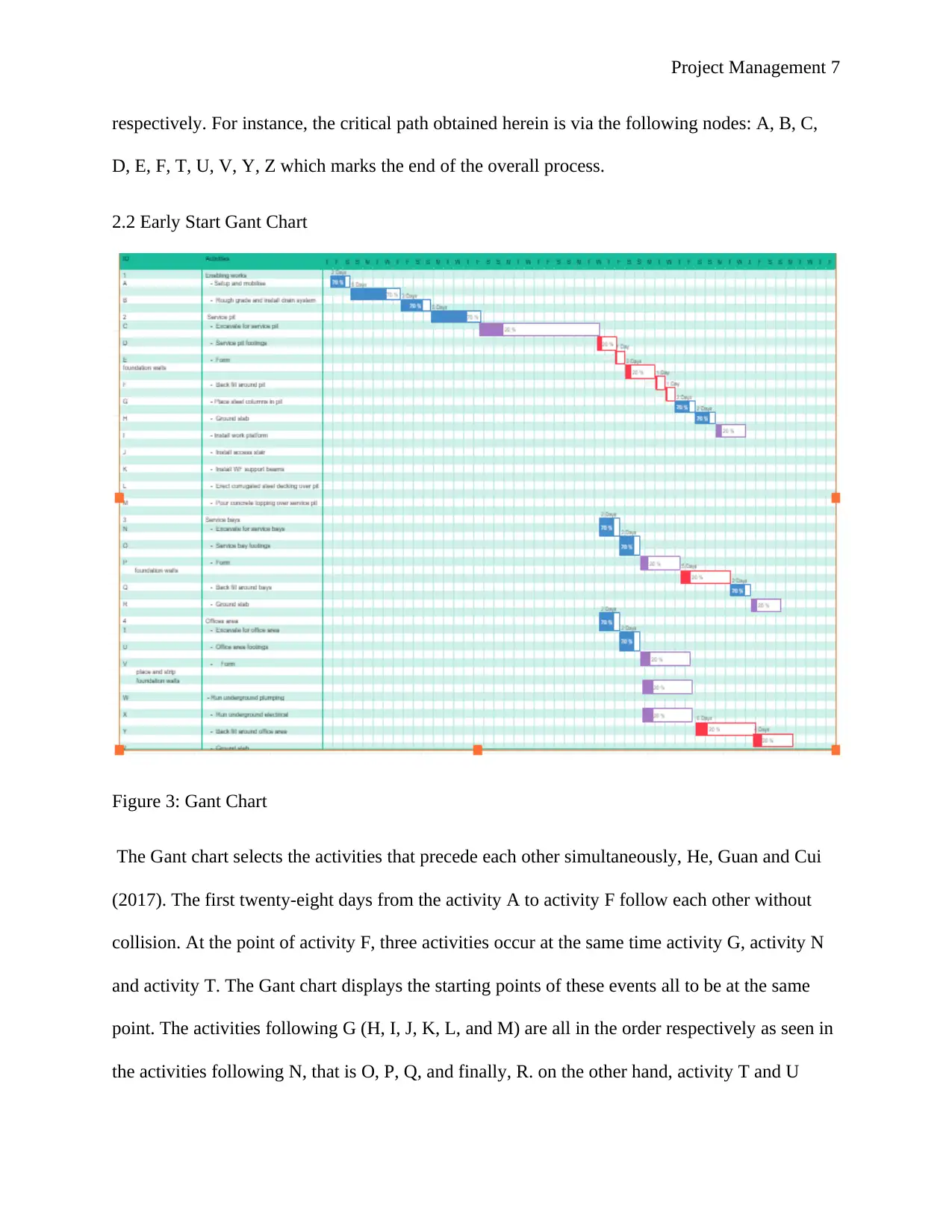
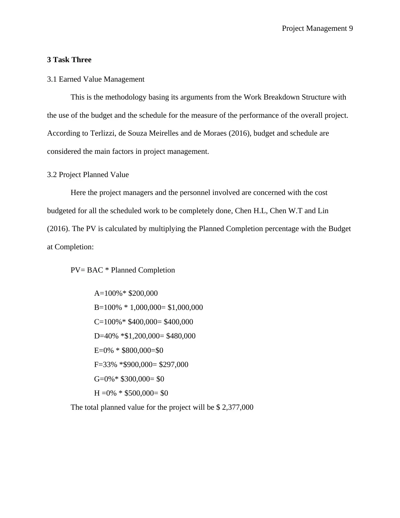
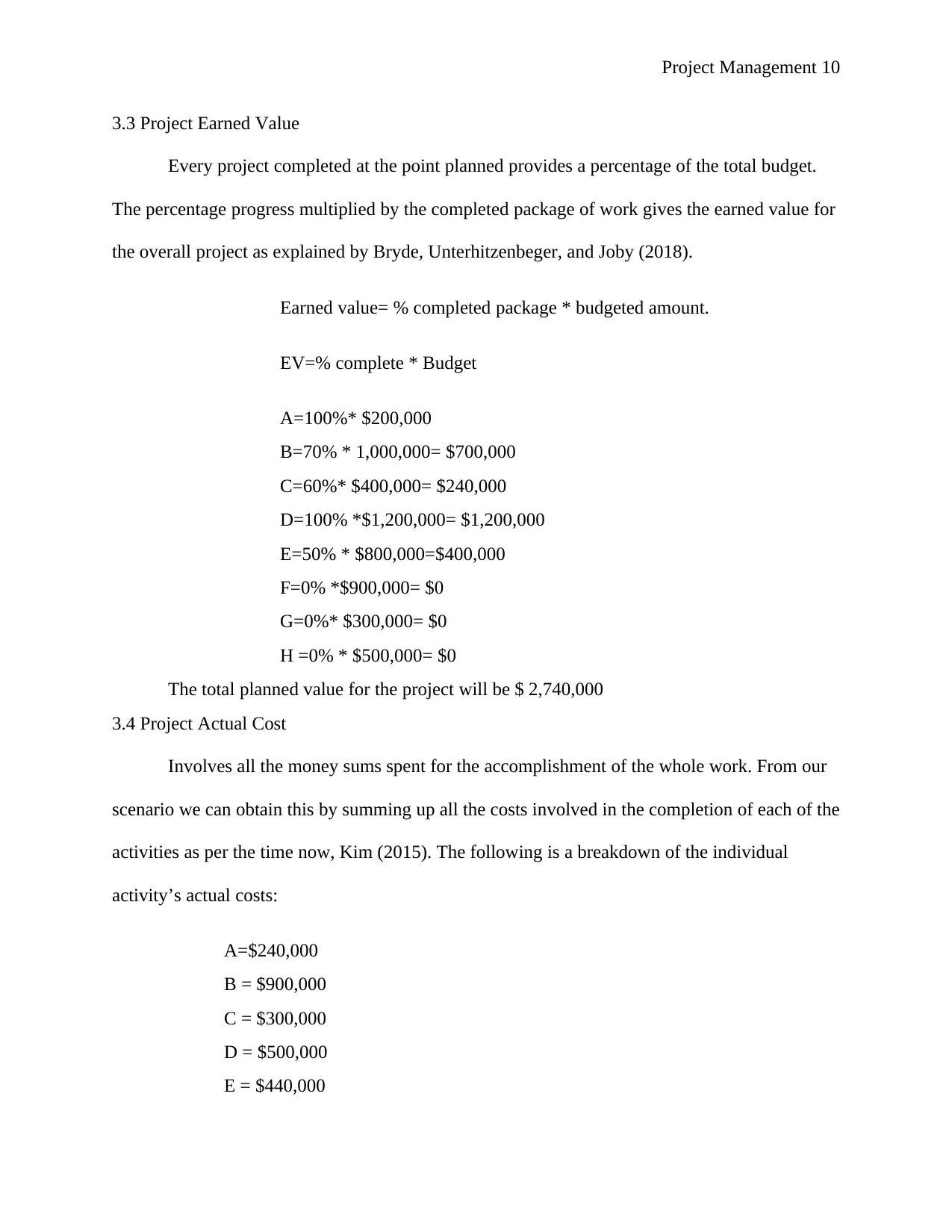
This project management assignment comprehensively addresses key concepts and methodologies in project management. It begins with a decision tree analysis, providing a framework for evaluating project choices and their associated risks and benefits. The assignment then proceeds to create an activity-on-node network diagram to illustrate project dependencies and critical paths, followed by the development of an early start Gantt chart for visual project scheduling. Furthermore, the assignment delves into earned value management (EVM), calculating planned value (PV), earned value (EV), actual cost (AC), cost variance (CV), and schedule variance (SV) to assess project performance. The analysis includes a project revised budget and detailed calculations for each component of EVM, offering a thorough understanding of project cost and schedule control. The report concludes with a discussion of the project's financial health and potential future outcomes based on the analysis.

Project Management 1
Project Management
Student Name
Course
Professor’s Name
Institution Name
Location of Institution
Date

Project Management 2
Project Management
Table of Contents
Abbreviations...................................................................................................................................3
List of Figures..................................................................................................................................3
1 Task One.......................................................................................................................................4
1.1 Decision Tree.........................................................................................................................4
1.2 Decision Tree Analysis..........................................................................................................4
2 Task Two......................................................................................................................................6
2.1 Activity on Node network diagram.......................................................................................6
2.2 Early Start Gant Chart...........................................................................................................7
2.3 Fifty Day Completion............................................................................................................8
3 Task Three....................................................................................................................................9
3.1 Earned Value Management....................................................................................................9
3.2 Project Planned Value............................................................................................................9
3.3 Project Earned Value.............................................................................................................9
3.4 Project Actual Cost..............................................................................................................10
3.5 Remaining Work Value.......................................................................................................11
3.6 Cost Variance and Schedule Variance.................................................................................11
3.7 Project Revised Budget........................................................................................................13
References......................................................................................................................................14

Project Management 3
Abbreviations
1. EVM –Earned Value Management
2. BCWS- Budgeted Cost of Work Schedule
3. BCWP- Budgeted Cost of Work Performed
4. BCWR- Budgeted Cost of Work Remaining
5. AC- Actual Cost
6. PV- Planned Value
7. EV- Earned Value
8. CV- Cost Variance
9. SV- Schedule Variance
10. BAC – Budget at Completion
11. ESS- Earliest Start Schedule
12. LSS- Latest Start Schedule
List of Figures
Figure 1: Decision Tree Diagram....................................................................................................5
Figure 2: Activity on Node network diagram..................................................................................6
Figure 3: Gant Chart........................................................................................................................7
13.

Project Management 4
1 Task One
1.1 Decision Tree
In every situation, we are faced with a dilemma in which we have a choice to pick from a
variety of options available. In this scenario, a decision tree diagram helps in mapping out all the
related series of the outcomes. With a mathematical influence, the decision tree diagram is based
on its algorithm in the probability of occurrence, the cost of the choice and the corresponding
benefit that comes along if it is chosen and all other risk associated, Webb (2017).
Figure 1: Decision Tree Diagram
1.2 Decision Tree Analysis
From the design above, the do-nothing option should not be given any attention since the
costs seem to be preferably higher though the benefits are directly propositional. Investing
happens to be the most profiting factor in any growing organization. In this review, a higher
percentage is given to the investment and this provides the basis for our decision. At this level,

Project Management 5
configurations and the repairs are brought on the table. Any spending on the repairs yields less
compared to the configurations.
Relocation and reconfiguration bring dilemma, both have a higher percentage in terms of
benefits hence brings forth a challenge to the project managers. Based on their timescales,
reconfiguration which requires only a year to be completed, outdo the latter and is given a
probability of 70 percent. Innovation and collaboration are well favored in this path and we
conclude that this becomes the best path to follow since its profits are higher compared to the
other provided options. In this research, the decision tree displays that with the booming
economy, there is a tremendous increase in the benefit realized from the first year and the second
year.

Project Management 6
2 Task Two
2.1 Activity on Node network diagram
Schedule activities can be easily identified in the project management task through the use of
these diagrams. Activities are connected together in a precedence format to show each of the
relationships that exist between two nodes and their dependencies. From the first activity, we get
to understand the activity that needs to be completed first before the commence of the other and
those that occur at the same time as seen in node G, node N, and node T.
Figure 2: Activity on Node network diagram
From the network diagram above, the calculation ESS and the LSS provides the overall
time taken for the whole project to be complete which is 49 days. The critical path is obtained by
the nodes having the same ESS and the LSS, the result of forward and backward calculations

Project Management 7
respectively. For instance, the critical path obtained herein is via the following nodes: A, B, C,
D, E, F, T, U, V, Y, Z which marks the end of the overall process.
2.2 Early Start Gant Chart
Figure 3: Gant Chart
The Gant chart selects the activities that precede each other simultaneously, He, Guan and Cui
(2017). The first twenty-eight days from the activity A to activity F follow each other without
collision. At the point of activity F, three activities occur at the same time activity G, activity N
and activity T. The Gant chart displays the starting points of these events all to be at the same
point. The activities following G (H, I, J, K, L, and M) are all in the order respectively as seen in
the activities following N, that is O, P, Q, and finally, R. on the other hand, activity T and U

Project Management 8
Follows F simultaneously. At point U three activities start at the same time, activity V, activity
W, and activity X. Activity Y follows V and immediately it comes to an end, we realize that W
and X will be also at its end, activity Z begins immediately all the three activities (Y, W, and X)
stops.
2.3 Fifty Day Completion
Given the activities D- service pit footings and Z- ground slap for the office area, we can
calculate the expected time for each as shown below.
Expected time = (Optimistic Time + 4 x Most likely Time + Pessimistic Time) / 6.
Expected time for activity D= ((4 + 4) * (5 +7))/ 6
= (8 * 12) / 6
= 96 / 6 =16 days
Expected time for activity Z= ((3 + 4) * (4 +8))/ 6
= (7 * 12) / 6
= 84 / 6 =14 days
Total expected time = (16 + 14) days
=30 days
Probability 30/50 =0.6 This is the probability that the project will be completed in 50 days.

Project Management 9
3 Task Three
3.1 Earned Value Management
This is the methodology basing its arguments from the Work Breakdown Structure with
the use of the budget and the schedule for the measure of the performance of the overall project.
According to Terlizzi, de Souza Meirelles and de Moraes (2016), budget and schedule are
considered the main factors in project management.
3.2 Project Planned Value
Here the project managers and the personnel involved are concerned with the cost
budgeted for all the scheduled work to be completely done, Chen H.L, Chen W.T and Lin
(2016). The PV is calculated by multiplying the Planned Completion percentage with the Budget
at Completion:
PV= BAC * Planned Completion
A=100%* $200,000
B=100% * 1,000,000= $1,000,000
C=100%* $400,000= $400,000
D=40% *$1,200,000= $480,000
E=0% * $800,000=$0
F=33% *$900,000= $297,000
G=0%* $300,000= $0
H =0% * $500,000= $0
The total planned value for the project will be $ 2,377,000

Project Management 10
3.3 Project Earned Value
Every project completed at the point planned provides a percentage of the total budget.
The percentage progress multiplied by the completed package of work gives the earned value for
the overall project as explained by Bryde, Unterhitzenbeger, and Joby (2018).
Earned value= % completed package * budgeted amount.
EV=% complete * Budget
A=100%* $200,000
B=70% * 1,000,000= $700,000
C=60%* $400,000= $240,000
D=100% *$1,200,000= $1,200,000
E=50% * $800,000=$400,000
F=0% *$900,000= $0
G=0%* $300,000= $0
H =0% * $500,000= $0
The total planned value for the project will be $ 2,740,000
3.4 Project Actual Cost
Involves all the money sums spent for the accomplishment of the whole work. From our
scenario we can obtain this by summing up all the costs involved in the completion of each of the
activities as per the time now, Kim (2015). The following is a breakdown of the individual
activity’s actual costs:
A=$240,000
B = $900,000
C = $300,000
D = $500,000
E = $440,000

Project Management 11
F = $0
G = $0
H = $0
Total = $ (240,000 + 900,000 + 300,000 + 500,000 + 440,000 + 0 + 0 + 0)
The total actual cost for the project is: $ 2 830,000
3.5 Remaining Work Value
This gives a representation of the budget portion for the work that has not yet been
accomplished, Torrecilla-Salinas, Sedeno, Escalona and Mejias (2015). It is simply displaying
the difference between the Budgeted cost at Completion and the overall cumulative cost budget
for work performed.
We obtain by the formula BCWR= BAC-BCWP
= $ (200,000 + 1,000,000 + 400,000 + 1,200,000 + 800,000 + 900,000 + 300,000 + 500,000)
= $ 5,300,000 -$ 2,377,000
=$ 2,923,000
3.6 Cost Variance and Schedule Variance
The difference between the actual amount of the cost and the planned amount results to a
Cost variance while the schedule variance indicates if the schedule for any project is ahead of
time or behind, Pheng (2018). We can calculate by obtaining the difference between the Budget
Cost of Work Performed and the Budgeted Cost of Work Scheduled.
CV= EV-AC
SV= BCWP – BCWS or the EV- PV
Let’s consider the Cost Variance and Schedule Variance for each of the activities:
Activity A

Project Management 12
Cost Variance Schedule Variance
AC=$240,000
EV= $200,000
CV= $200,000- $240,000 = -$40,000
PV=$200,000
EV= $200,000
SV= $200,000- $200,000 = $0
Activity B
Cost Variance Schedule Variance
AC=$900,000
EV= 70/100 * $1,000,000= $700,000
CV= $700,000- $900,000 = -$200,000
PV=$1,000,000
EV= $700,000
SV= $700,000- $1,000,000 = -$300,000
Activity C
Cost Variance Schedule Variance
AC=$300,000
EV= 60/100 * $400,000= $240,000
CV= $240,000- $300,000 = -$60,000
PV=$400,000
EV= 60/100 * $400,000= $240,000
SV= $240,000- $400,000 = -$160,000
Activity D
Cost Variance Schedule Variance
AC=$500,000
EV= 100/100 * $1,200,000= $1,200,000
CV= $1,200,000- $500,000 = $700,000
PV=40/100* 1,200,000=$480,000
EV= 100/100 * $1,200,000= $1,200,000
SV= $1,200,000- $480,000 = $720,000
Activity E
Cost Variance Schedule Variance
AC=$440,000
EV= 50/100 * $800,000= $400,000
CV= $400,000 - $440,000 = -$40,000
PV=$400,000
EV= 0/100 * $800,000= $0
SV= $400,000 - $0 = $400,000
Activity F