Decision Analysis, Value of Information, Monte Carlo Simulation, Regression Analysis

This article covers topics such as decision analysis, value of information, Monte Carlo simulation, and regression analysis. It includes examples and explanations of each topic.

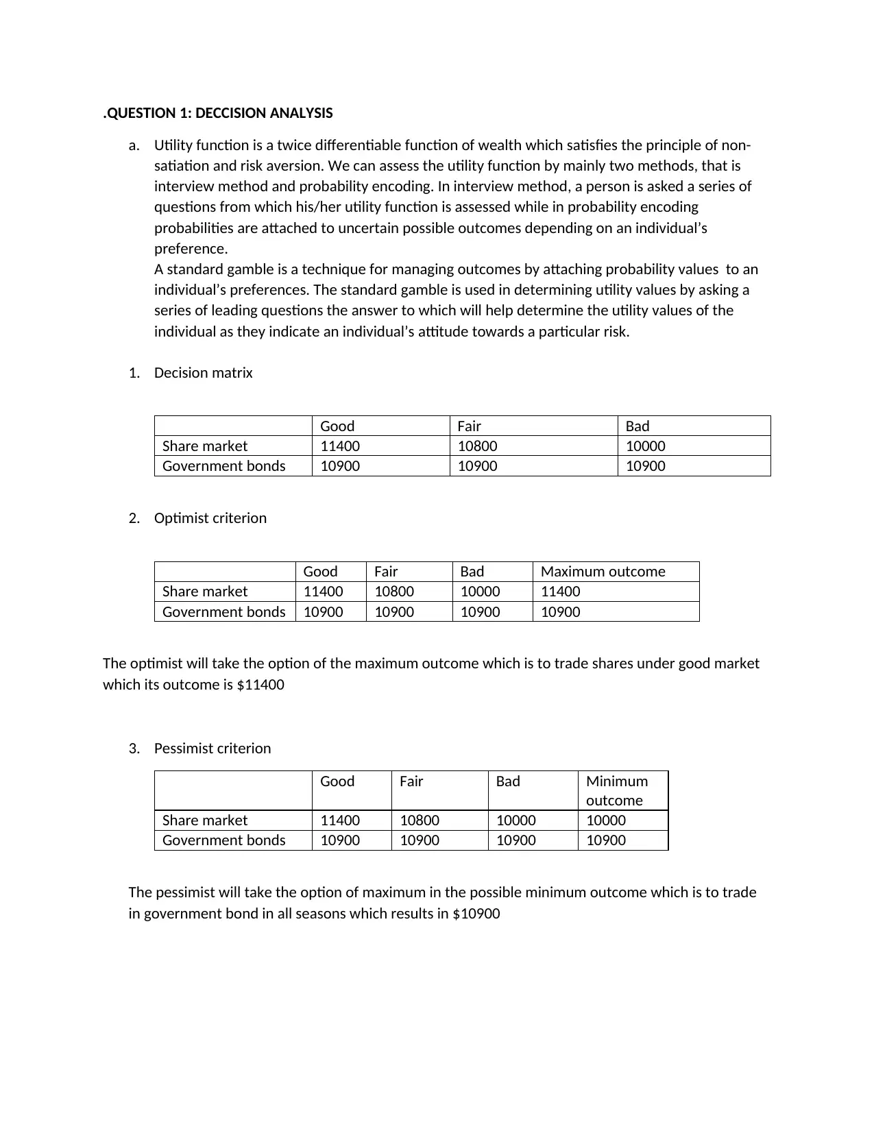
.QUESTION 1: DECCISION ANALYSIS
a. Utility function is a twice differentiable function of wealth which satisfies the principle of non-
satiation and risk aversion. We can assess the utility function by mainly two methods, that is
interview method and probability encoding. In interview method, a person is asked a series of
questions from which his/her utility function is assessed while in probability encoding
probabilities are attached to uncertain possible outcomes depending on an individual’s
preference.
A standard gamble is a technique for managing outcomes by attaching probability values to an
individual’s preferences. The standard gamble is used in determining utility values by asking a
series of leading questions the answer to which will help determine the utility values of the
individual as they indicate an individual’s attitude towards a particular risk.
1. Decision matrix
Good Fair Bad
Share market 11400 10800 10000
Government bonds 10900 10900 10900
2. Optimist criterion
Good Fair Bad Maximum outcome
Share market 11400 10800 10000 11400
Government bonds 10900 10900 10900 10900
The optimist will take the option of the maximum outcome which is to trade shares under good market
which its outcome is $11400
3. Pessimist criterion
Good Fair Bad Minimum
outcome
Share market 11400 10800 10000 10000
Government bonds 10900 10900 10900 10900
The pessimist will take the option of maximum in the possible minimum outcome which is to trade
in government bond in all seasons which results in $10900

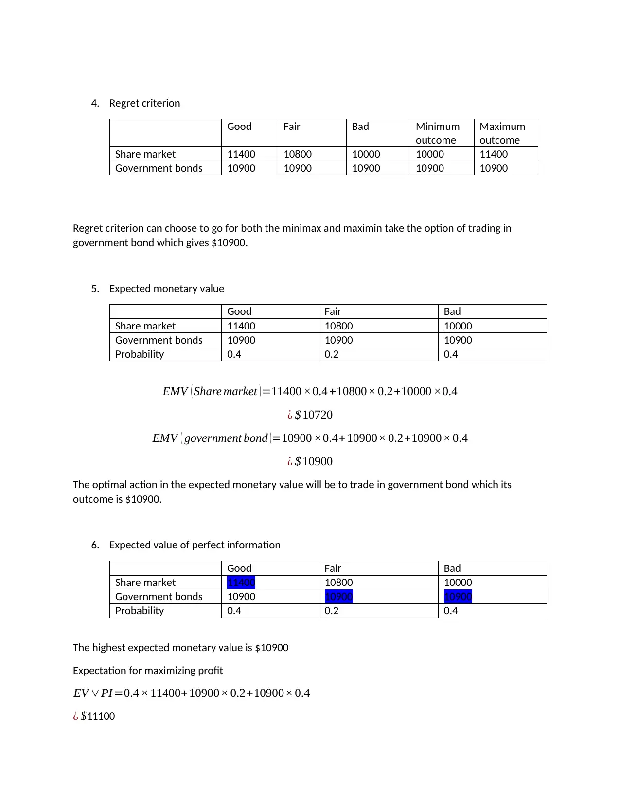
4. Regret criterion
Good Fair Bad Minimum
outcome
Maximum
outcome
Share market 11400 10800 10000 10000 11400
Government bonds 10900 10900 10900 10900 10900
Regret criterion can choose to go for both the minimax and maximin take the option of trading in
government bond which gives $10900.
5. Expected monetary value
Good Fair Bad
Share market 11400 10800 10000
Government bonds 10900 10900 10900
Probability 0.4 0.2 0.4
EMV ( Share market )=11400 ×0.4 +10800× 0.2+10000 ×0.4
¿ $ 10720
EMV ( government bond )=10900 ×0.4+ 10900× 0.2+10900× 0.4
¿ $ 10900
The optimal action in the expected monetary value will be to trade in government bond which its
outcome is $10900.
6. Expected value of perfect information
Good Fair Bad
Share market 11400 10800 10000
Government bonds 10900 10900 10900
Probability 0.4 0.2 0.4
The highest expected monetary value is $10900
Expectation for maximizing profit
EV ∨PI =0.4 × 11400+ 10900× 0.2+10900× 0.4
¿ $11100

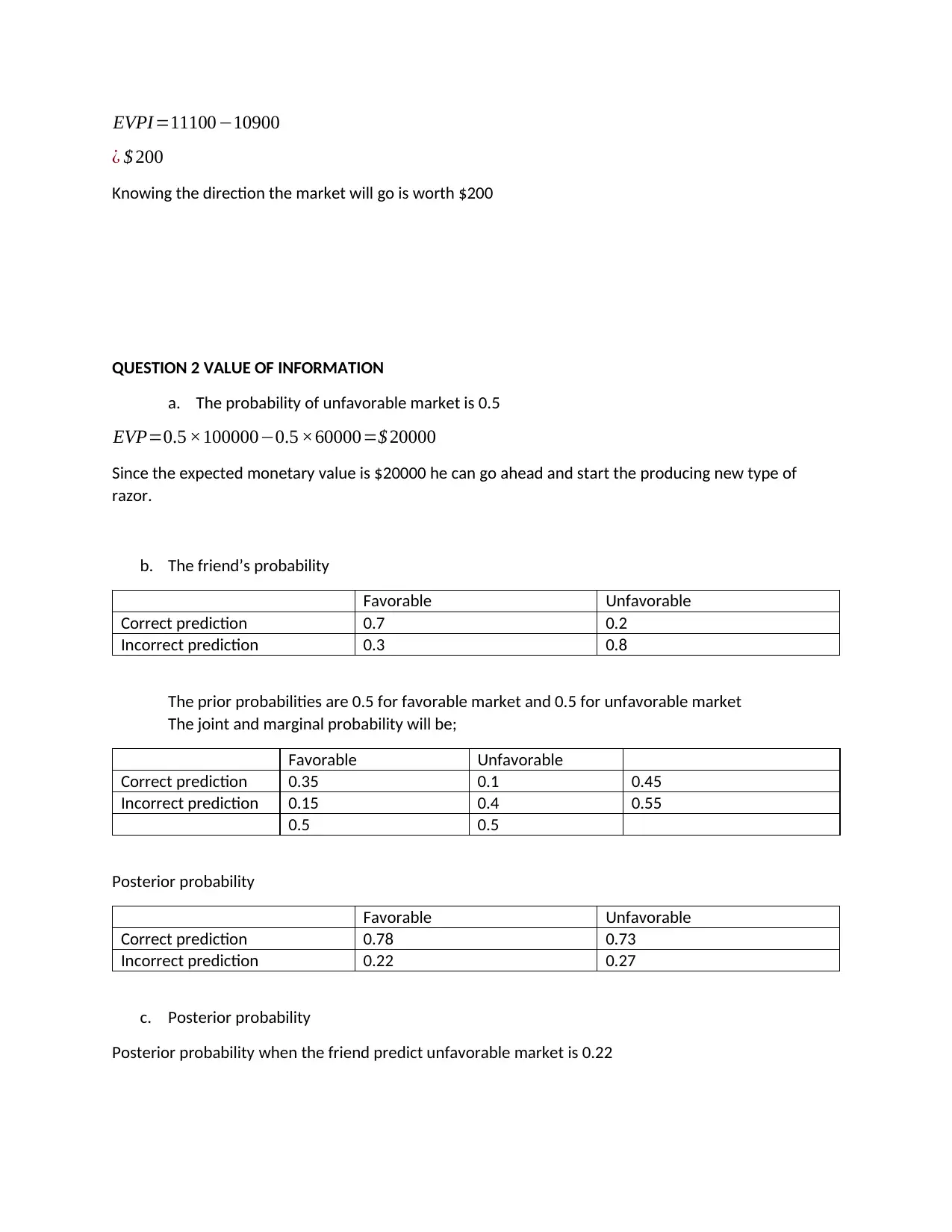
EVPI=11100−10900
¿ $ 200
Knowing the direction the market will go is worth $200
QUESTION 2 VALUE OF INFORMATION
a. The probability of unfavorable market is 0.5
EVP=0.5 ×100000−0.5 ×60000=$ 20000
Since the expected monetary value is $20000 he can go ahead and start the producing new type of
razor.
b. The friend’s probability
Favorable Unfavorable
Correct prediction 0.7 0.2
Incorrect prediction 0.3 0.8
The prior probabilities are 0.5 for favorable market and 0.5 for unfavorable market
The joint and marginal probability will be;
Favorable Unfavorable
Correct prediction 0.35 0.1 0.45
Incorrect prediction 0.15 0.4 0.55
0.5 0.5
Posterior probability
Favorable Unfavorable
Correct prediction 0.78 0.73
Incorrect prediction 0.22 0.27
c. Posterior probability
Posterior probability when the friend predict unfavorable market is 0.22

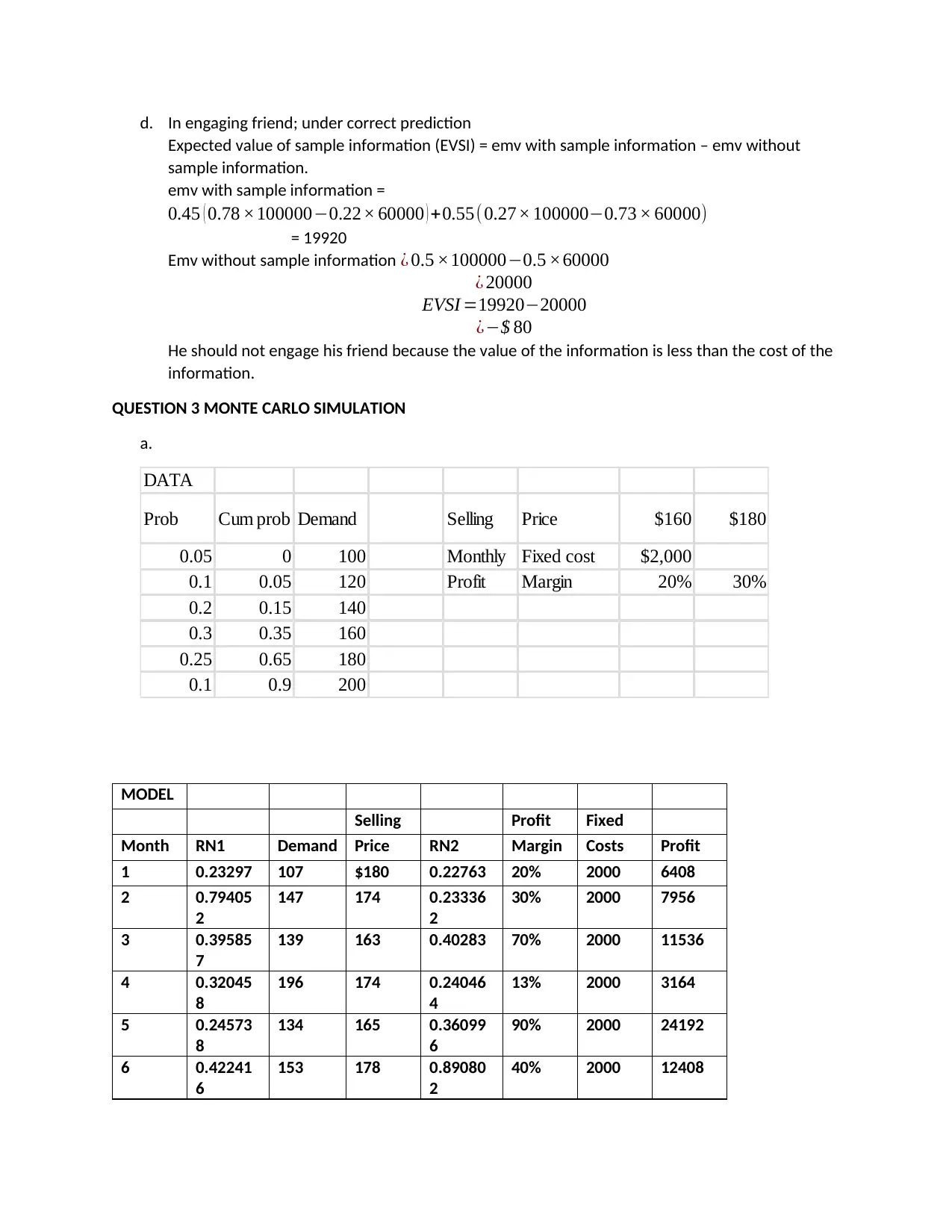
d. In engaging friend; under correct prediction
Expected value of sample information (EVSI) = emv with sample information – emv without
sample information.
emv with sample information =
0.45 ( 0.78 ×100000−0.22× 60000 ) +0.55(0.27× 100000−0.73 × 60000)
= 19920
Emv without sample information ¿ 0.5 ×100000−0.5 ×60000
¿ 20000
EVSI =19920−20000
¿−$ 80
He should not engage his friend because the value of the information is less than the cost of the
information.
QUESTION 3 MONTE CARLO SIMULATION
a.
DATA
Prob Cum prob Demand Selling Price $160 $180
0.05 0 100 Monthly Fixed cost $2,000
0.1 0.05 120 Profit Margin 20% 30%
0.2 0.15 140
0.3 0.35 160
0.25 0.65 180
0.1 0.9 200
MODEL
Selling Profit Fixed
Month RN1 Demand Price RN2 Margin Costs Profit
1 0.23297 107 $180 0.22763 20% 2000 6408
2 0.79405
2
147 174 0.23336
2
30% 2000 7956
3 0.39585
7
139 163 0.40283 70% 2000 11536
4 0.32045
8
196 174 0.24046
4
13% 2000 3164
5 0.24573
8
134 165 0.36099
6
90% 2000 24192
6 0.42241
6
153 178 0.89080
2
40% 2000 12408

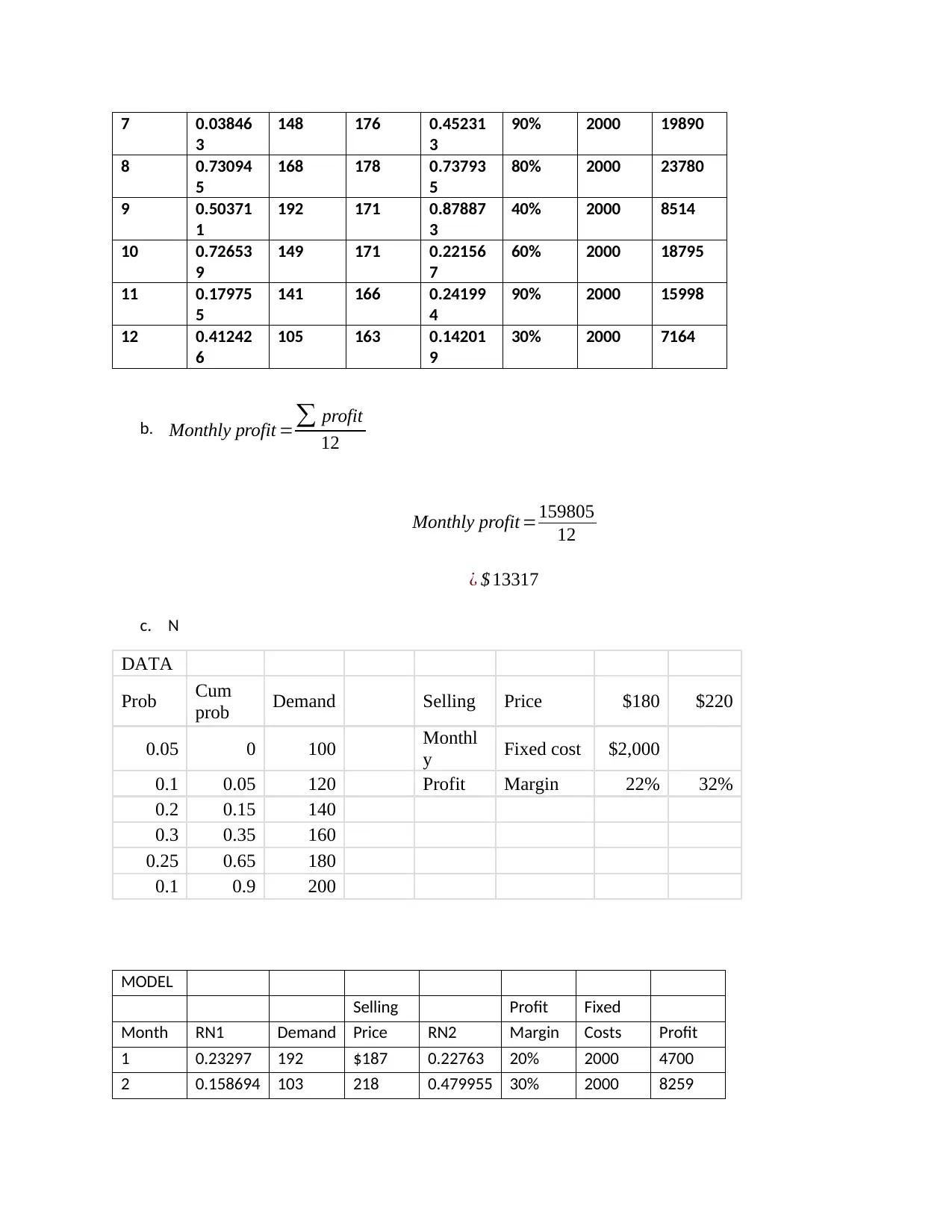
7 0.03846
3
148 176 0.45231
3
90% 2000 19890
8 0.73094
5
168 178 0.73793
5
80% 2000 23780
9 0.50371
1
192 171 0.87887
3
40% 2000 8514
10 0.72653
9
149 171 0.22156
7
60% 2000 18795
11 0.17975
5
141 166 0.24199
4
90% 2000 15998
12 0.41242
6
105 163 0.14201
9
30% 2000 7164
b. Monthly profit =∑ profit
12
Monthly profit =159805
12
¿ $ 13317
c. N
DATA
Prob Cum
prob Demand Selling Price $180 $220
0.05 0 100 Monthl
y Fixed cost $2,000
0.1 0.05 120 Profit Margin 22% 32%
0.2 0.15 140
0.3 0.35 160
0.25 0.65 180
0.1 0.9 200
MODEL
Selling Profit Fixed
Month RN1 Demand Price RN2 Margin Costs Profit
1 0.23297 192 $187 0.22763 20% 2000 4700
2 0.158694 103 218 0.479955 30% 2000 8259

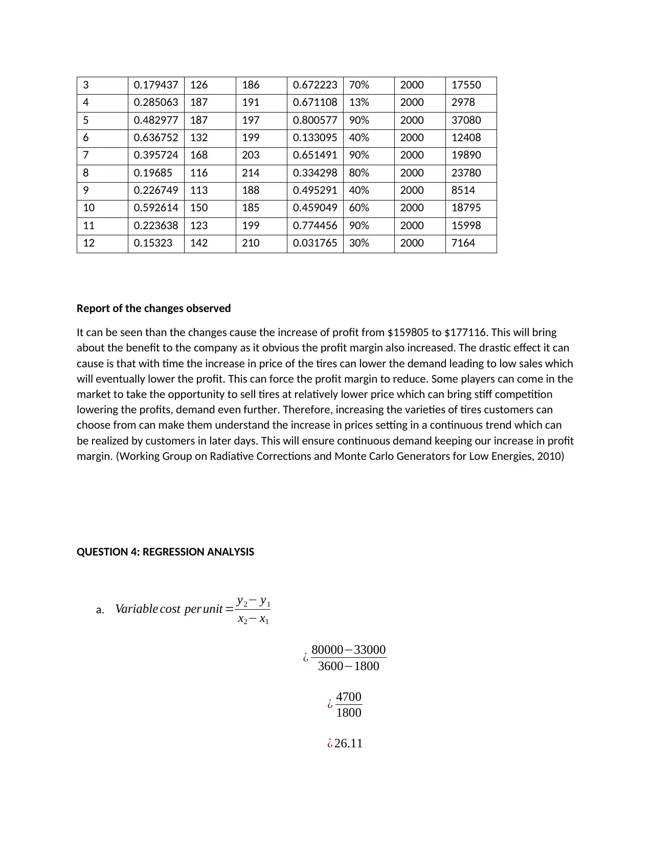
3 0.179437 126 186 0.672223 70% 2000 17550
4 0.285063 187 191 0.671108 13% 2000 2978
5 0.482977 187 197 0.800577 90% 2000 37080
6 0.636752 132 199 0.133095 40% 2000 12408
7 0.395724 168 203 0.651491 90% 2000 19890
8 0.19685 116 214 0.334298 80% 2000 23780
9 0.226749 113 188 0.495291 40% 2000 8514
10 0.592614 150 185 0.459049 60% 2000 18795
11 0.223638 123 199 0.774456 90% 2000 15998
12 0.15323 142 210 0.031765 30% 2000 7164
Report of the changes observed
It can be seen than the changes cause the increase of profit from $159805 to $177116. This will bring
about the benefit to the company as it obvious the profit margin also increased. The drastic effect it can
cause is that with time the increase in price of the tires can lower the demand leading to low sales which
will eventually lower the profit. This can force the profit margin to reduce. Some players can come in the
market to take the opportunity to sell tires at relatively lower price which can bring stiff competition
lowering the profits, demand even further. Therefore, increasing the varieties of tires customers can
choose from can make them understand the increase in prices setting in a continuous trend which can
be realized by customers in later days. This will ensure continuous demand keeping our increase in profit
margin. (Working Group on Radiative Corrections and Monte Carlo Generators for Low Energies, 2010)
QUESTION 4: REGRESSION ANALYSIS
a. Variable cost per unit = y2− y1
x2− x1
¿ 80000−33000
3600−1800
¿ 4700
1800
¿ 26.11

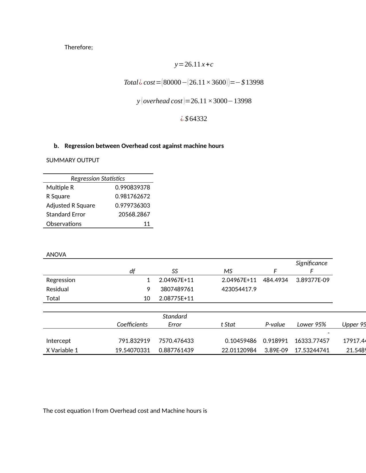
Therefore;
y=26.11 x +c
Total ¿ cost= ( 80000− ( 26.11× 3600 ) )=−$ 13998
y ( overhead cost )=26.11 ×3000−13998
¿ $ 64332
b. Regression between Overhead cost against machine hours
SUMMARY OUTPUT
Regression Statistics
Multiple R 0.990839378
R Square 0.981762672
Adjusted R Square 0.979736303
Standard Error 20568.2867
Observations 11
ANOVA
df SS MS F
Significance
F
Regression 1 2.04967E+11 2.04967E+11 484.4934 3.89377E-09
Residual 9 3807489761 423054417.9
Total 10 2.08775E+11
Coefficients
Standard
Error t Stat P-value Lower 95% Upper 95
Intercept 791.832919 7570.476433 0.10459486 0.918991
-
16333.77457 17917.44
X Variable 1 19.54070331 0.887761439 22.01120984 3.89E-09 17.53244741 21.5489
The cost equation I from Overhead cost and Machine hours is

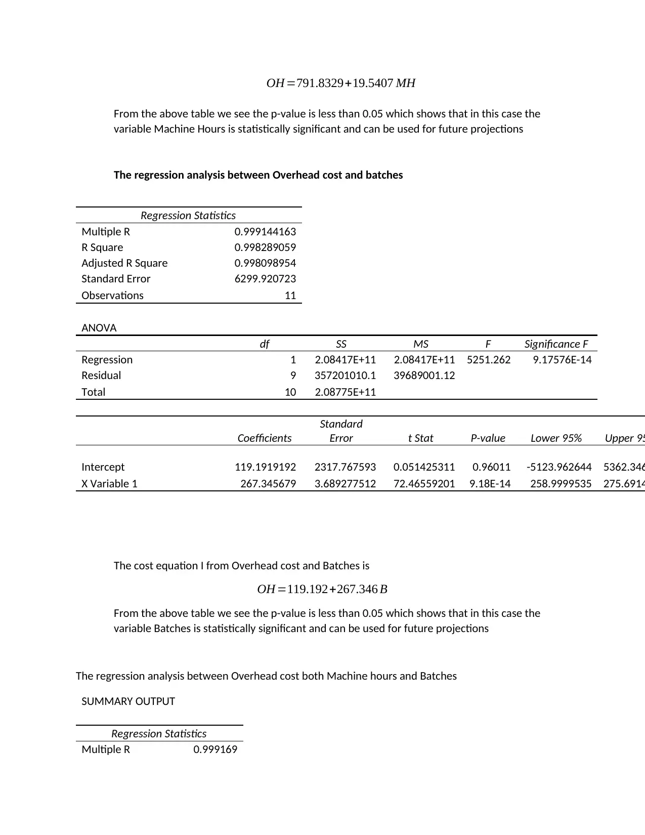
OH =791.8329+19.5407 MH
From the above table we see the p-value is less than 0.05 which shows that in this case the
variable Machine Hours is statistically significant and can be used for future projections
The regression analysis between Overhead cost and batches
Regression Statistics
Multiple R 0.999144163
R Square 0.998289059
Adjusted R Square 0.998098954
Standard Error 6299.920723
Observations 11
ANOVA
df SS MS F Significance F
Regression 1 2.08417E+11 2.08417E+11 5251.262 9.17576E-14
Residual 9 357201010.1 39689001.12
Total 10 2.08775E+11
Coefficients
Standard
Error t Stat P-value Lower 95% Upper 95
Intercept 119.1919192 2317.767593 0.051425311 0.96011 -5123.962644 5362.346
X Variable 1 267.345679 3.689277512 72.46559201 9.18E-14 258.9999535 275.6914
The cost equation I from Overhead cost and Batches is
OH =119.192+267.346 B
From the above table we see the p-value is less than 0.05 which shows that in this case the
variable Batches is statistically significant and can be used for future projections
The regression analysis between Overhead cost both Machine hours and Batches
SUMMARY OUTPUT
Regression Statistics
Multiple R 0.999169

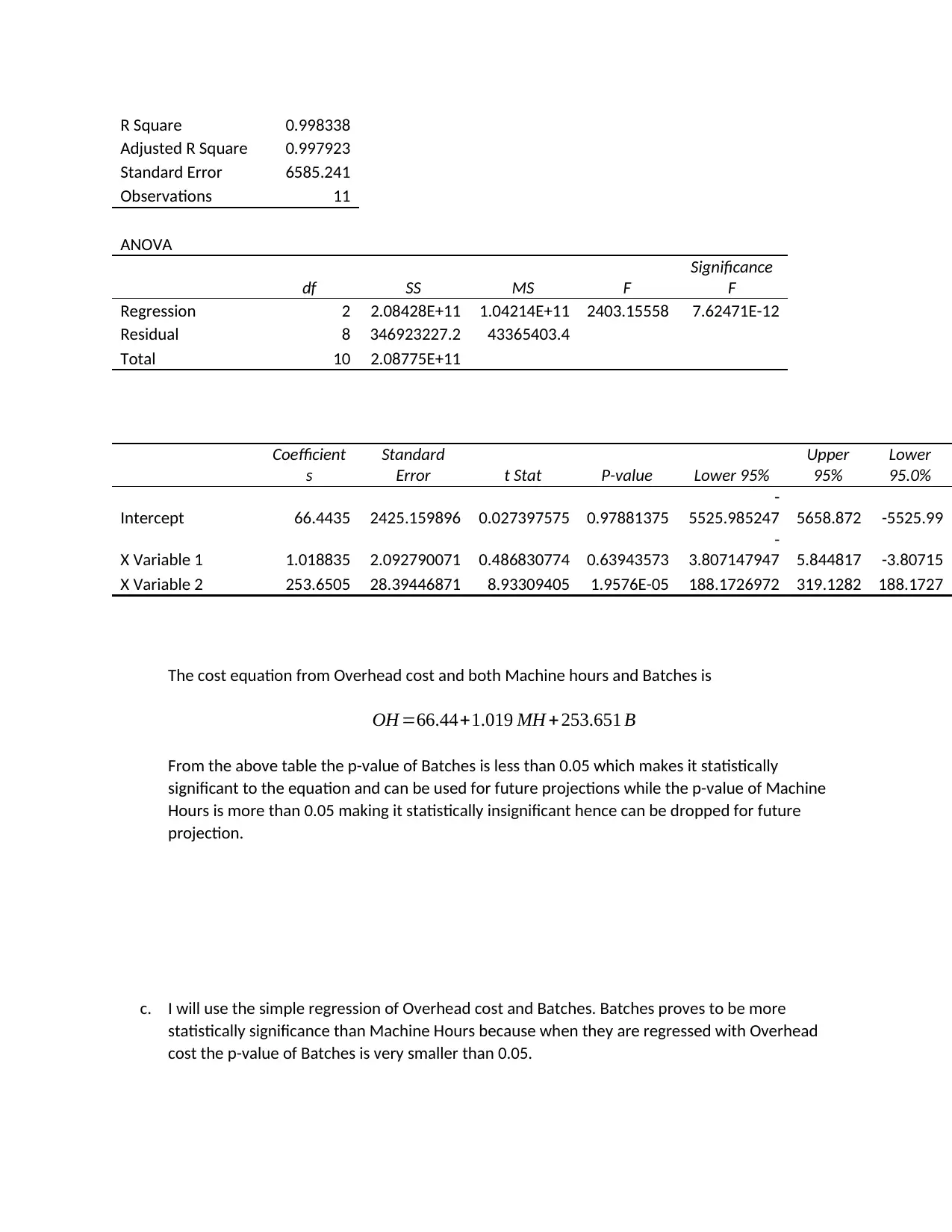
R Square 0.998338
Adjusted R Square 0.997923
Standard Error 6585.241
Observations 11
ANOVA
df SS MS F
Significance
F
Regression 2 2.08428E+11 1.04214E+11 2403.15558 7.62471E-12
Residual 8 346923227.2 43365403.4
Total 10 2.08775E+11
Coefficient
s
Standard
Error t Stat P-value Lower 95%
Upper
95%
Lower
95.0%
Intercept 66.4435 2425.159896 0.027397575 0.97881375
-
5525.985247 5658.872 -5525.99
X Variable 1 1.018835 2.092790071 0.486830774 0.63943573
-
3.807147947 5.844817 -3.80715
X Variable 2 253.6505 28.39446871 8.93309405 1.9576E-05 188.1726972 319.1282 188.1727
The cost equation from Overhead cost and both Machine hours and Batches is
OH =66.44+1.019 MH + 253.651 B
From the above table the p-value of Batches is less than 0.05 which makes it statistically
significant to the equation and can be used for future projections while the p-value of Machine
Hours is more than 0.05 making it statistically insignificant hence can be dropped for future
projection.
c. I will use the simple regression of Overhead cost and Batches. Batches proves to be more
statistically significance than Machine Hours because when they are regressed with Overhead
cost the p-value of Batches is very smaller than 0.05.

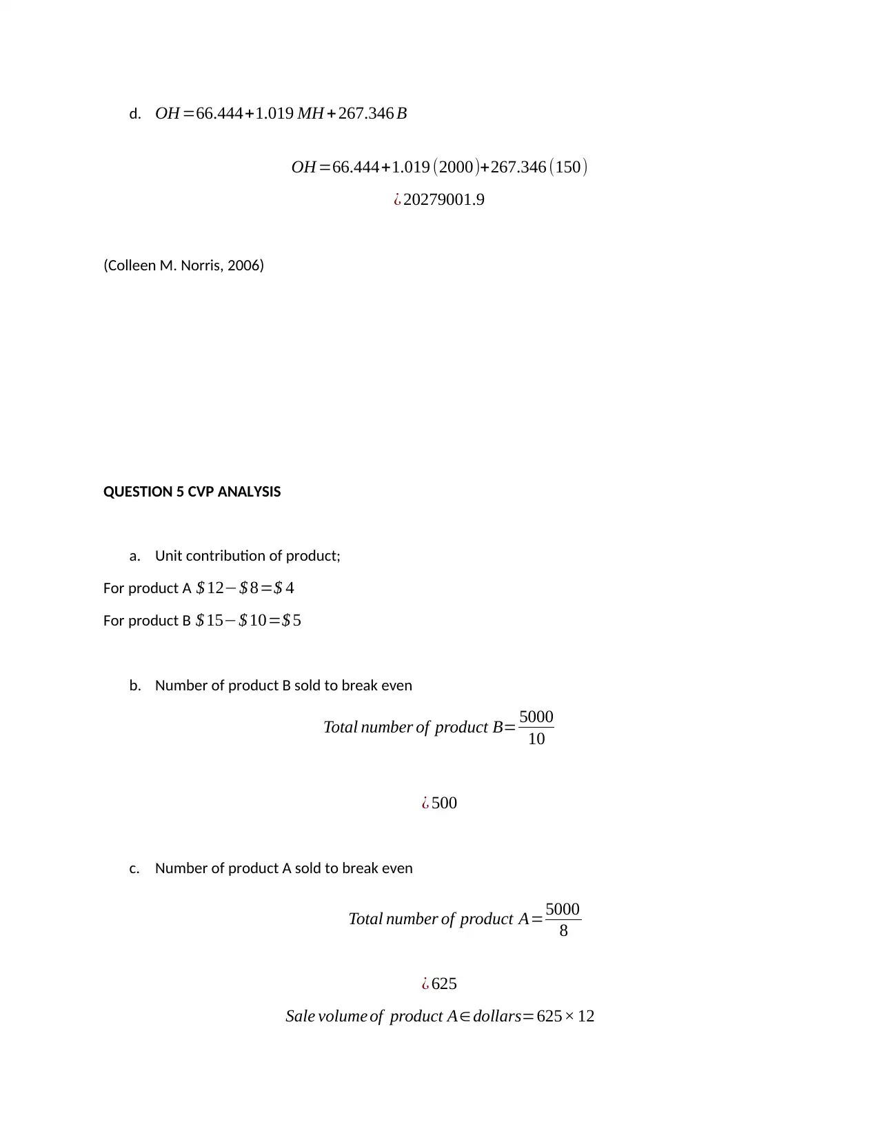
d. OH =66.444+1.019 MH + 267.346 B
OH =66.444+1.019 (2000)+267.346 (150)
¿ 20279001.9
(Colleen M. Norris, 2006)
QUESTION 5 CVP ANALYSIS
a. Unit contribution of product;
For product A $ 12−$ 8=$ 4
For product B $ 15−$ 10=$ 5
b. Number of product B sold to break even
Total number of product B= 5000
10
¿ 500
c. Number of product A sold to break even
Total number of product A=5000
8
¿ 625
Sale volume of product A∈dollars=625× 12

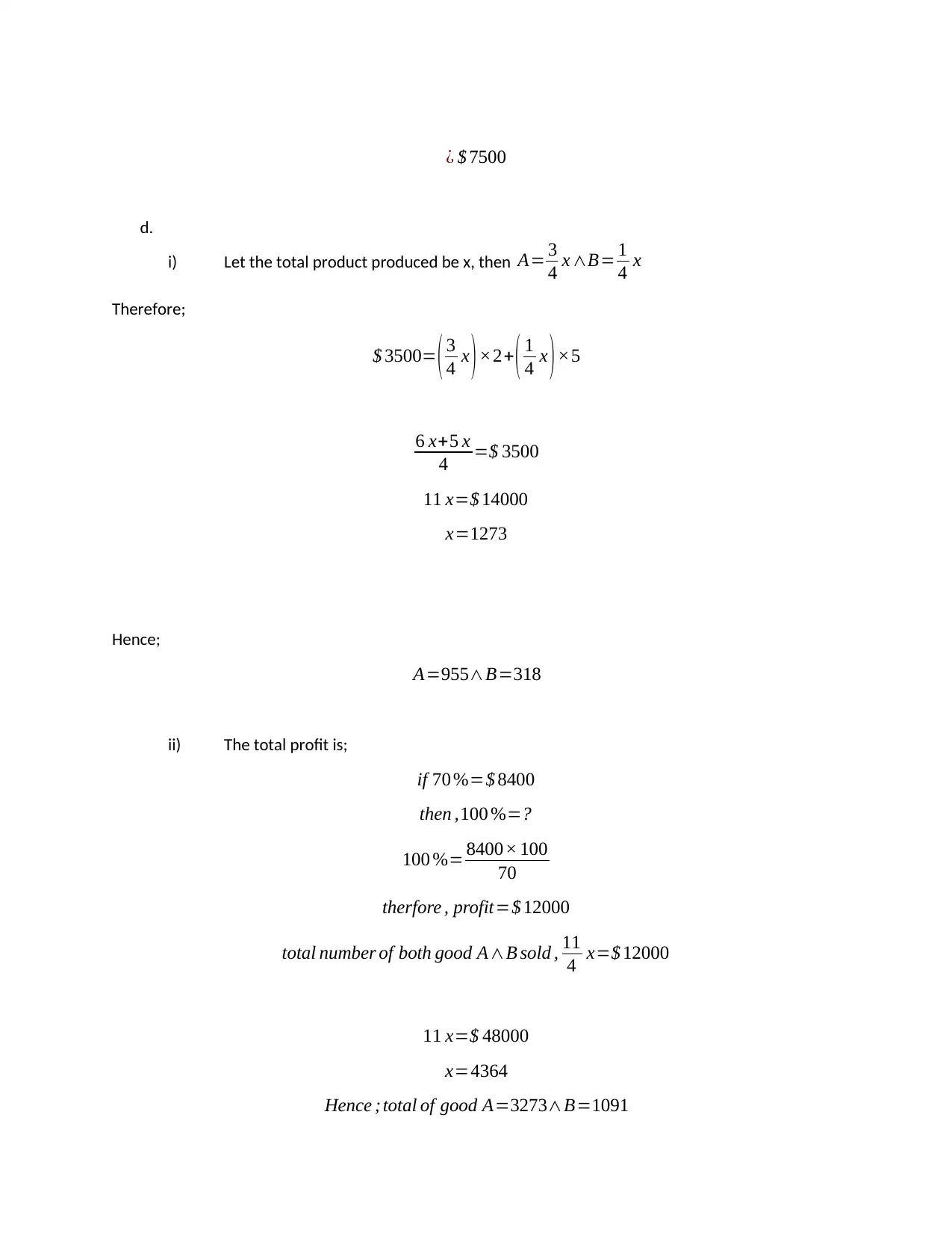
¿ $ 7500
d.
i) Let the total product produced be x, then A= 3
4 x ∧B= 1
4 x
Therefore;
$ 3500= ( 3
4 x )×2+ ( 1
4 x )×5
6 x+5 x
4 =$ 3500
11 x=$ 14000
x=1273
Hence;
A=955∧B=318
ii) The total profit is;
if 70 %=$ 8400
then ,100 %=?
100 %= 8400× 100
70
therfore , profit=$ 12000
total number of both good A∧B sold , 11
4 x=$ 12000
11 x=$ 48000
x=4364
Hence ; total of good A=3273∧B=1091

References
Colleen M. Norris, W. A. (2006). Ordinal regression model and the linear regression model were superior
to the logistic regression models. 9.
Working Group on Radiative Corrections and Monte Carlo Generators for Low Energies, S. A. (2010).
Quest for precision in hadronic cross sections at low energy:. Monte Carlo tools vs. experimental
data, 102.