Demand and Forecasting

This chapter discusses the growth of transportation modes in the tourism industry. It includes plotting raw data and logarithm of arrivals for each transportation mode against time, creating an index number to represent the growth of arrivals in each transportation mode, and formulating a model of passenger arrival data on cruise ships over time. The chapter concludes with a discussion on whether a nonlinear or linear model would be preferable for passenger arrivals by ferry against time.

RUNNING HEADER: DEMAND AND FORECASTING 1
Demand and Forecasting
Students name:
Students ID:
Institution:

Demand and Forecasting 2
Chapter 5
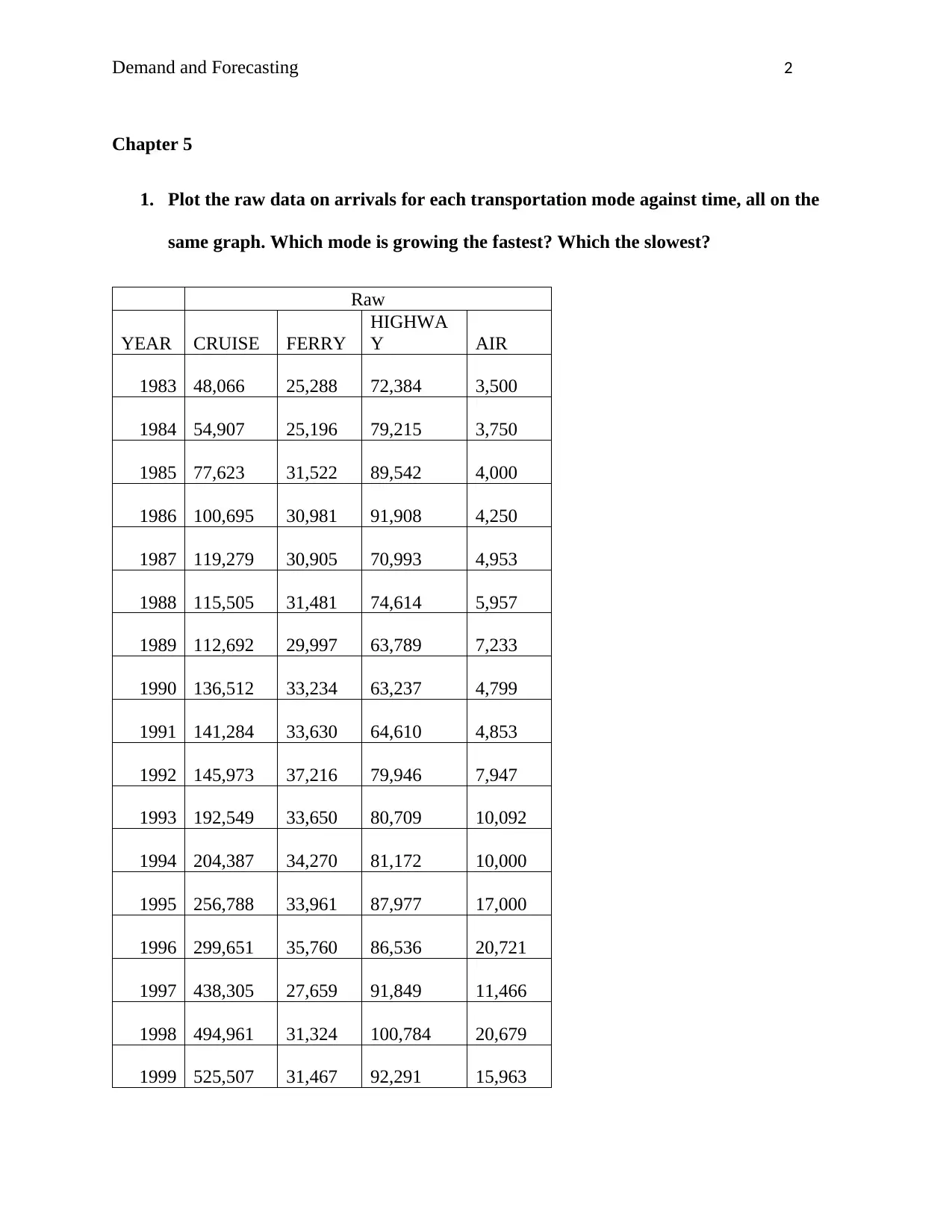
1. Plot the raw data on arrivals for each transportation mode against time, all on the
same graph. Which mode is growing the fastest? Which the slowest?
Raw
YEAR CRUISE FERRY
HIGHWA
Y AIR
1983 48,066 25,288 72,384 3,500
1984 54,907 25,196 79,215 3,750
1985 77,623 31,522 89,542 4,000
1986 100,695 30,981 91,908 4,250
1987 119,279 30,905 70,993 4,953
1988 115,505 31,481 74,614 5,957
1989 112,692 29,997 63,789 7,233
1990 136,512 33,234 63,237 4,799
1991 141,284 33,630 64,610 4,853
1992 145,973 37,216 79,946 7,947
1993 192,549 33,650 80,709 10,092
1994 204,387 34,270 81,172 10,000
1995 256,788 33,961 87,977 17,000
1996 299,651 35,760 86,536 20,721
1997 438,305 27,659 91,849 11,466
1998 494,961 31,324 100,784 20,679
1999 525,507 31,467 92,291 15,963

Demand and Forecasting 3
1983 1984 1985 1986 1987 1988 1989 1990 1991 1992 1993 1994 1995 1996 1997 1998 1999
-
100,000
200,000
300,000
400,000
500,000
600,000
Chart Title
CRUISE FERRY HIGHWAY AIR
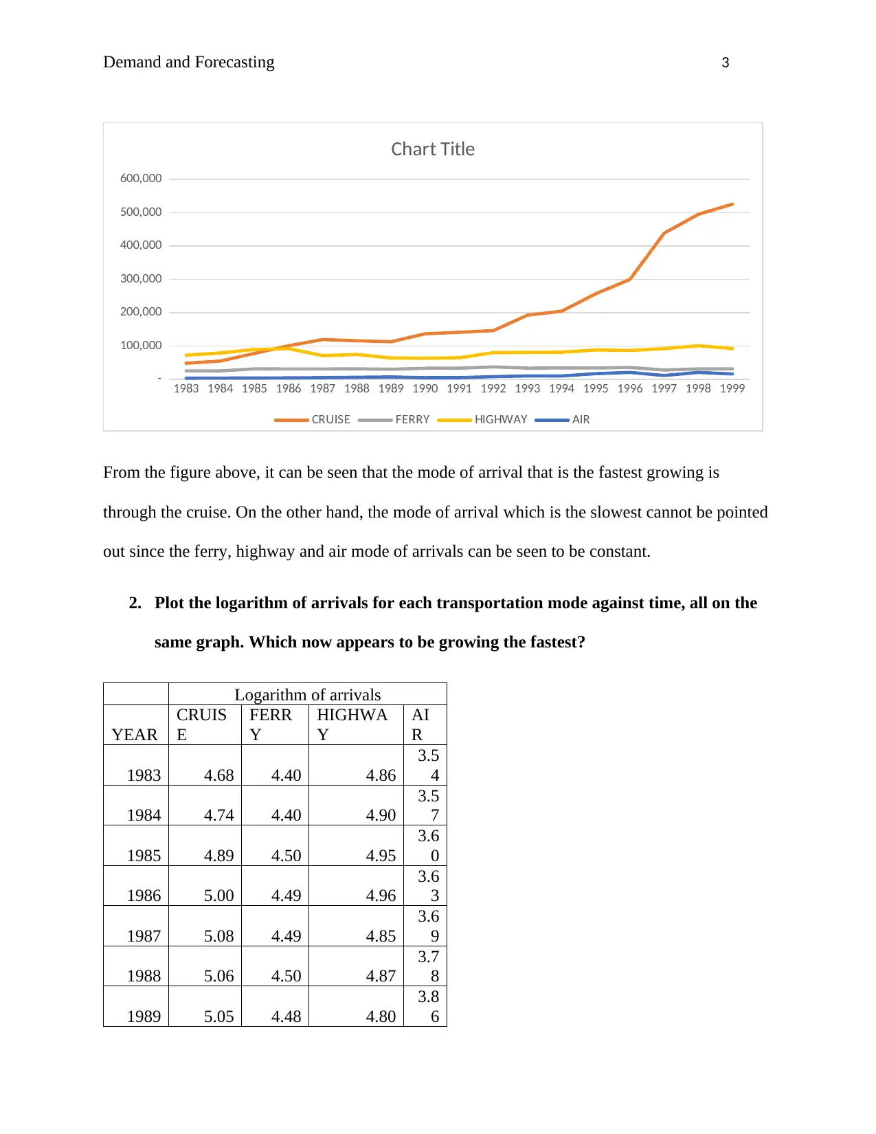
From the figure above, it can be seen that the mode of arrival that is the fastest growing is
through the cruise. On the other hand, the mode of arrival which is the slowest cannot be pointed
out since the ferry, highway and air mode of arrivals can be seen to be constant.
2. Plot the logarithm of arrivals for each transportation mode against time, all on the
same graph. Which now appears to be growing the fastest?
Logarithm of arrivals
YEAR
CRUIS
E
FERR
Y
HIGHWA
Y
AI
R
1983 4.68 4.40 4.86
3.5
4
1984 4.74 4.40 4.90
3.5
7
1985 4.89 4.50 4.95
3.6
0
1986 5.00 4.49 4.96
3.6
3
1987 5.08 4.49 4.85
3.6
9
1988 5.06 4.50 4.87
3.7
8
1989 5.05 4.48 4.80
3.8
6

Demand and Forecasting 4
1990 5.14 4.52 4.80
3.6
8
1991 5.15 4.53 4.81
3.6
9
1992 5.16 4.57 4.90
3.9
0
1993 5.28 4.53 4.91
4.0
0
1994 5.31 4.53 4.91
4.0
0
1995 5.41 4.53 4.94
4.2
3
1996 5.48 4.55 4.94
4.3
2
1997 5.64 4.44 4.96
4.0
6
1998 5.69 4.50 5.00
4.3
2
1999 5.72 4.50 4.97
4.2
0
1983 1984 1985 1986 1987 1988 1989 1990 1991 1992 1993 1994 1995 1996 1997 1998 1999
0.00
1.00
2.00
3.00
4.00
5.00
6.00
7.00
Chart Title
CRUISE FERRY HIGHWAY AIR
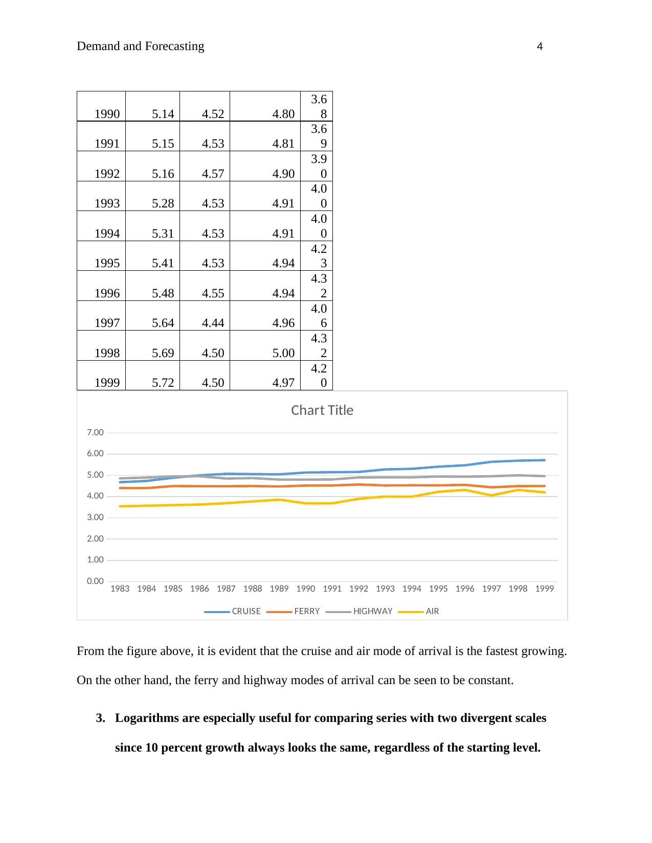
From the figure above, it is evident that the cruise and air mode of arrival is the fastest growing.
On the other hand, the ferry and highway modes of arrival can be seen to be constant.
3. Logarithms are especially useful for comparing series with two divergent scales
since 10 percent growth always looks the same, regardless of the starting level.

Demand and Forecasting 5
When absolute levels matter, the raw data are more appropriate, but when growth
rates are what’s important, log scales are better.
This is true as can be seen in question 1 and question 2. In question 2, it was seen that there was
growth in all the four modes of arrival whether positive or negative over time. On the other hand,
in absolute levels matter, only growth rate could be seen for the cruise mode of arrival while the
other 3 modes of arrival could be seen to be almost constant.
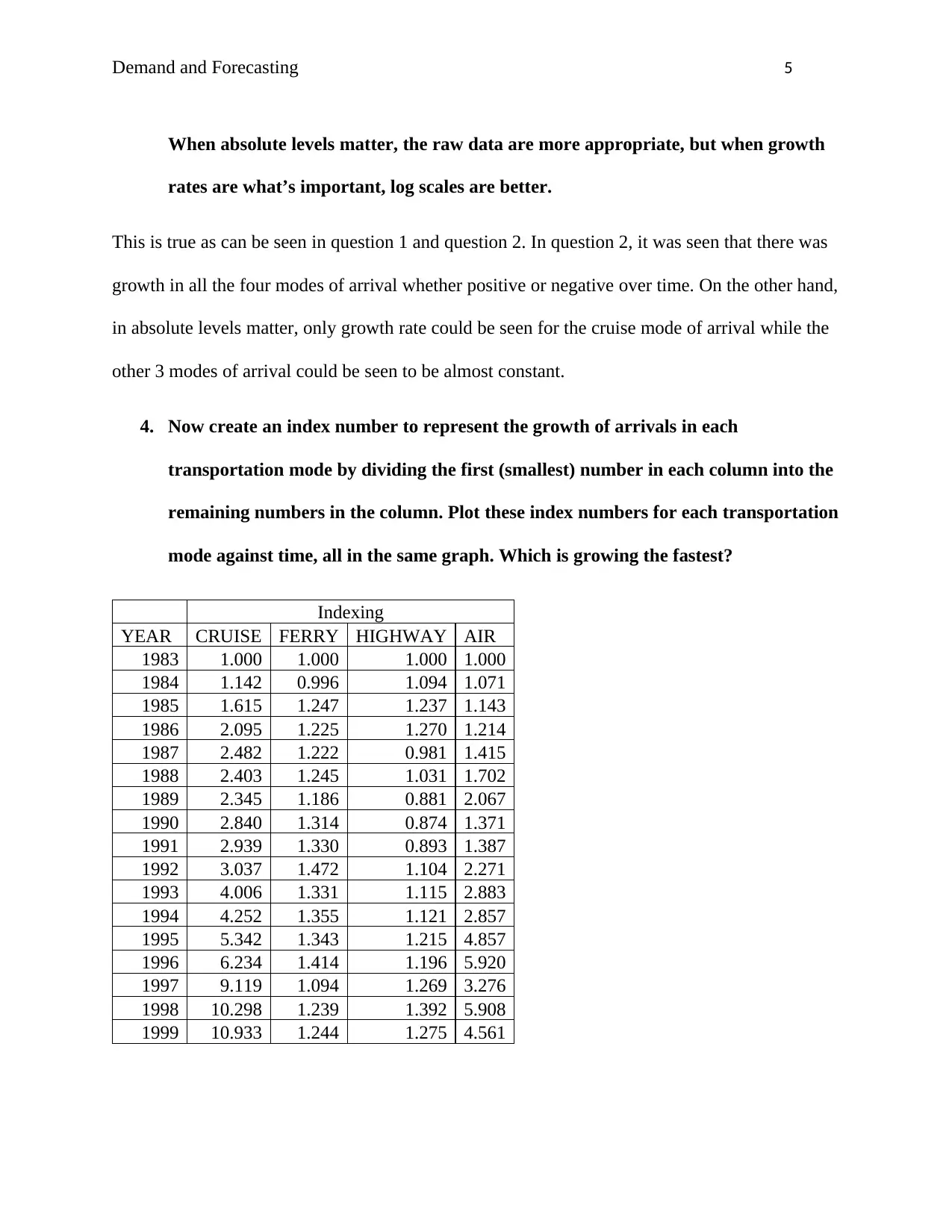
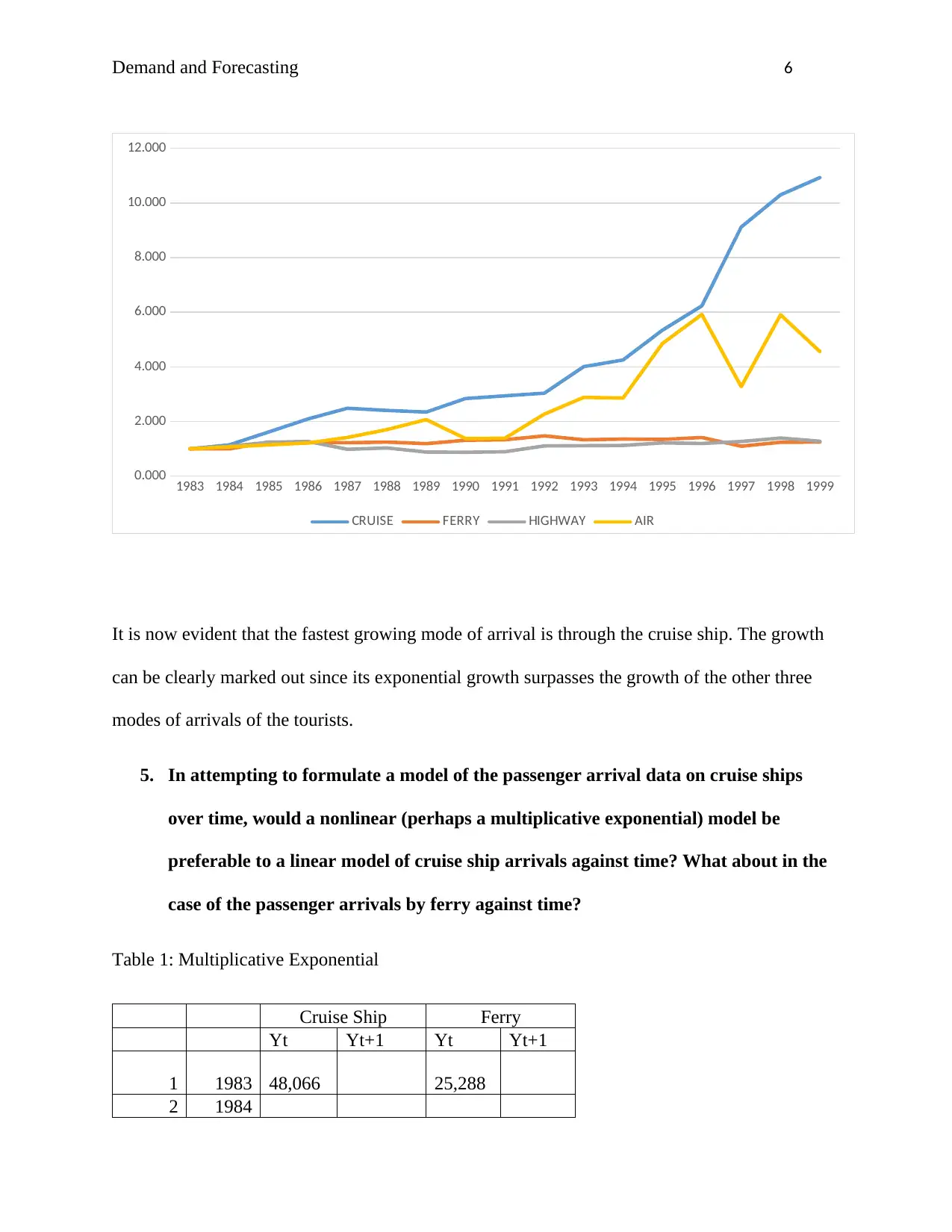
4. Now create an index number to represent the growth of arrivals in each
transportation mode by dividing the first (smallest) number in each column into the
remaining numbers in the column. Plot these index numbers for each transportation
mode against time, all in the same graph. Which is growing the fastest?
Indexing
YEAR CRUISE FERRY HIGHWAY AIR
1983 1.000 1.000 1.000 1.000
1984 1.142 0.996 1.094 1.071
1985 1.615 1.247 1.237 1.143
1986 2.095 1.225 1.270 1.214
1987 2.482 1.222 0.981 1.415
1988 2.403 1.245 1.031 1.702
1989 2.345 1.186 0.881 2.067
1990 2.840 1.314 0.874 1.371
1991 2.939 1.330 0.893 1.387
1992 3.037 1.472 1.104 2.271
1993 4.006 1.331 1.115 2.883
1994 4.252 1.355 1.121 2.857
1995 5.342 1.343 1.215 4.857
1996 6.234 1.414 1.196 5.920
1997 9.119 1.094 1.269 3.276
1998 10.298 1.239 1.392 5.908
1999 10.933 1.244 1.275 4.561

Demand and Forecasting 6
1983 1984 1985 1986 1987 1988 1989 1990 1991 1992 1993 1994 1995 1996 1997 1998 1999
0.000
2.000
4.000
6.000
8.000
10.000
12.000
CRUISE FERRY HIGHWAY AIR
It is now evident that the fastest growing mode of arrival is through the cruise ship. The growth
can be clearly marked out since its exponential growth surpasses the growth of the other three
modes of arrivals of the tourists.
5. In attempting to formulate a model of the passenger arrival data on cruise ships
over time, would a nonlinear (perhaps a multiplicative exponential) model be
preferable to a linear model of cruise ship arrivals against time? What about in the
case of the passenger arrivals by ferry against time?
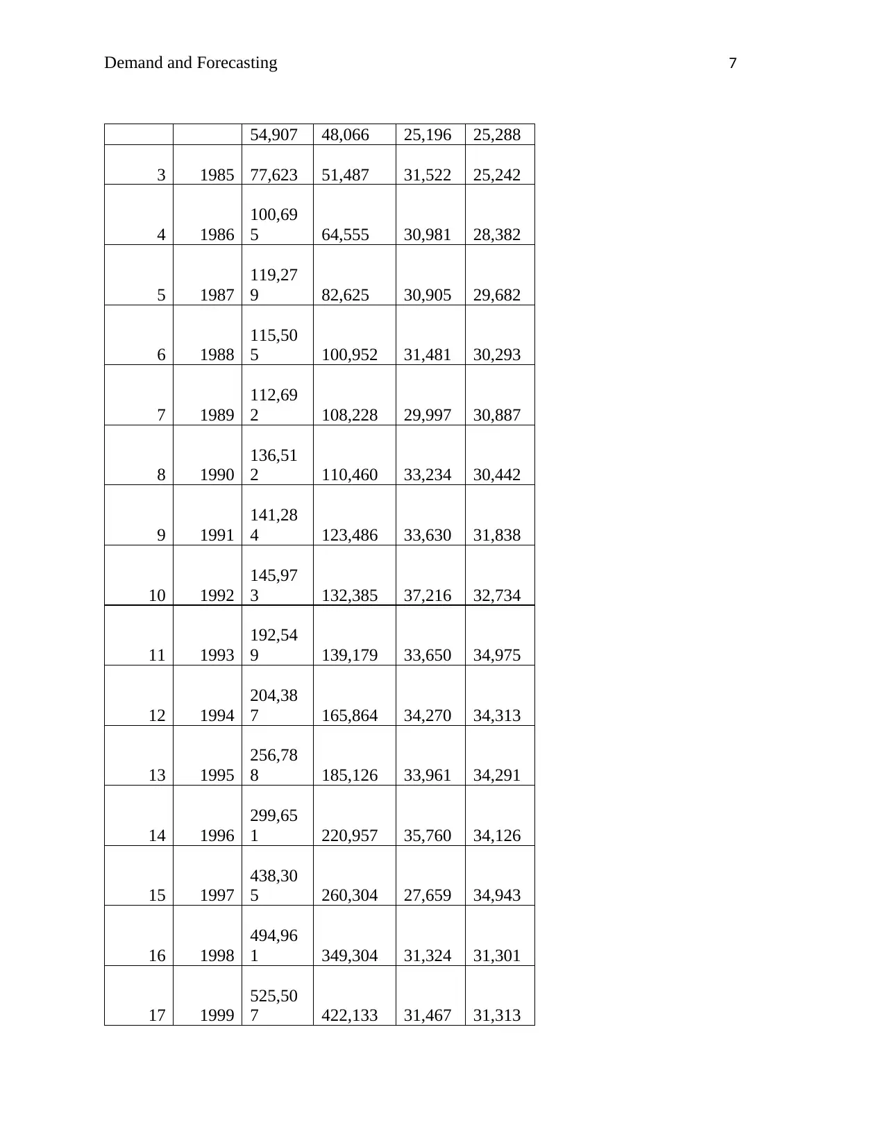
Table 1: Multiplicative Exponential
Cruise Ship Ferry
Yt Yt+1 Yt Yt+1
1 1983 48,066 25,288
2 1984

Demand and Forecasting 7
54,907 48,066 25,196 25,288
3 1985 77,623 51,487 31,522 25,242
4 1986
100,69
5 64,555 30,981 28,382
5 1987
119,27
9 82,625 30,905 29,682
6 1988
115,50
5 100,952 31,481 30,293
7 1989
112,69
2 108,228 29,997 30,887
8 1990
136,51
2 110,460 33,234 30,442
9 1991
141,28
4 123,486 33,630 31,838
10 1992
145,97
3 132,385 37,216 32,734
11 1993
192,54
9 139,179 33,650 34,975
12 1994
204,38
7 165,864 34,270 34,313
13 1995
256,78
8 185,126 33,961 34,291
14 1996
299,65
1 220,957 35,760 34,126
15 1997
438,30
5 260,304 27,659 34,943
16 1998
494,96
1 349,304 31,324 31,301
17 1999
525,50
7 422,133 31,467 31,313

Demand and Forecasting 8
1 2 3 4 5 6 7 8 9 10 11 12 13 14 15 16 17
-
50,000
100,000
150,000
200,000
250,000
300,000
350,000
400,000
450,000
Cruise Ship Yt+1 Ferry Yt+1
Cruise Ship Ferry
Yt Yt+1 Yt Yt+1
1 1983 48,066 75,136.18 25,288
25,594.1
9
2 1984 54,907
102,206.3
7 25,196
25,900.3
7
3 1985 77,623
129,276.5
5 31,522
26,206.5
6
4 1986
100,69
5
156,346.7
4 30,981
26,512.7
5
5 1987
119,27
9
183,416.9
2 30,905
26,818.9
3
6 1988
115,50
5
210,487.1
0 31,481
27,125.1
2
7 1989
112,69
2
237,557.2
9 29,997
27,431.3
0
8 1990
136,51 264,627.4 33,234 27,737.4

Demand and Forecasting 9
2 7 9
9 1991
141,28
4
291,697.6
5 33,630
28,043.6
8
10 1992
145,97
3
318,767.8
4 37,216
28,349.8
6
11 1993
192,54
9
345,838.0
2 33,650
28,656.0
5
12 1994
204,38
7
372,908.2
1 34,270
28,962.2
4
13 1995
256,78
8
399,978.3
9 33,961
29,268.4
2
14 1996
299,65
1
427,048.5
7 35,760
29,574.6
1
15 1997
438,30
5
454,118.7
6 27,659
29,880.7
9
16 1998
494,96
1
481,188.9
4 31,324
30,186.9
8
17 1999
525,50
7
508,259.1
3 31,467
30,493.1
7
Slope 27,070 306

Demand and Forecasting 10
1 2 3 4 5 6 7 8 9 10 11 12 13 14 15 16 17
-
100,000.00
200,000.00
300,000.00
400,000.00
500,000.00
600,000.00
Cruise Ship Yt+1 Ferry Yt+1
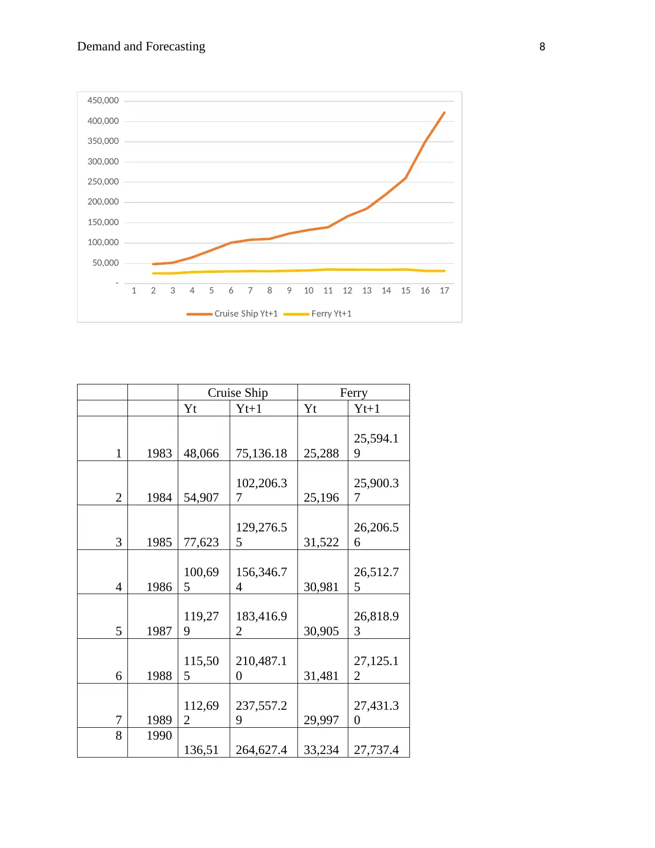
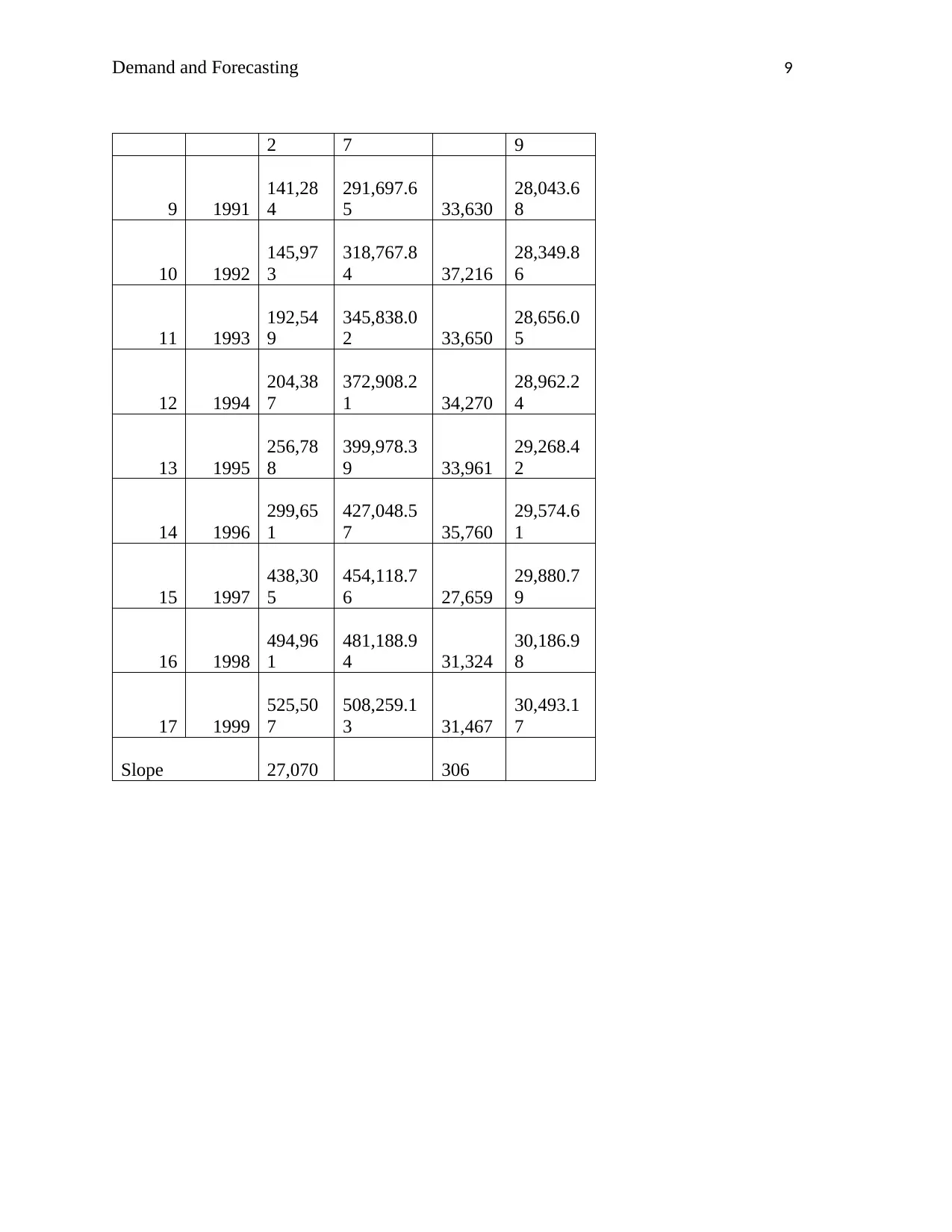
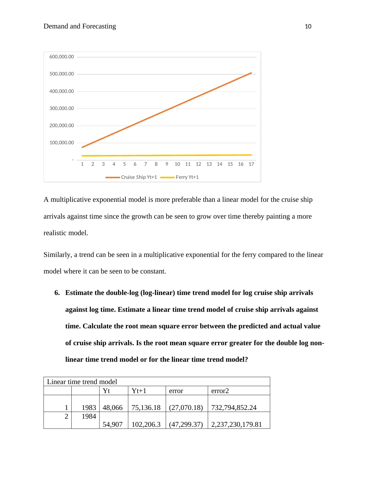
A multiplicative exponential model is more preferable than a linear model for the cruise ship
arrivals against time since the growth can be seen to grow over time thereby painting a more
realistic model.
Similarly, a trend can be seen in a multiplicative exponential for the ferry compared to the linear
model where it can be seen to be constant.
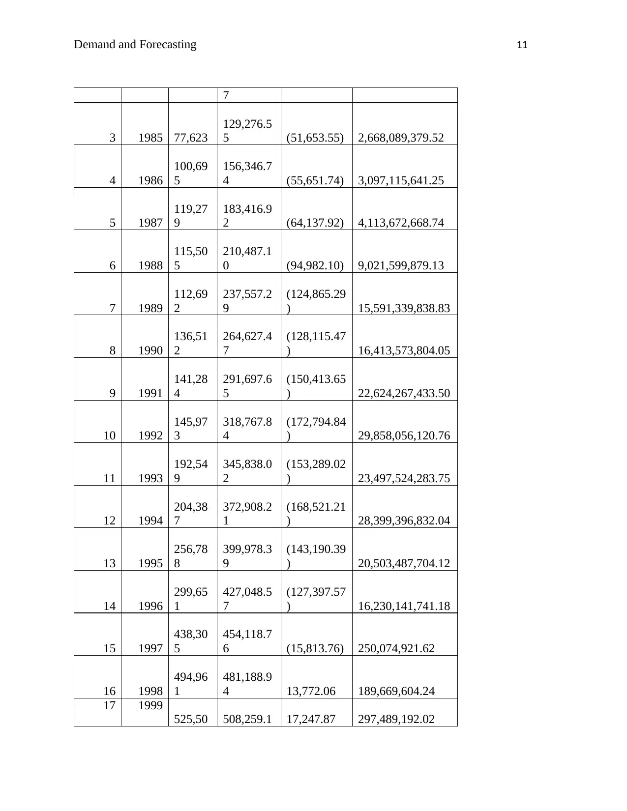
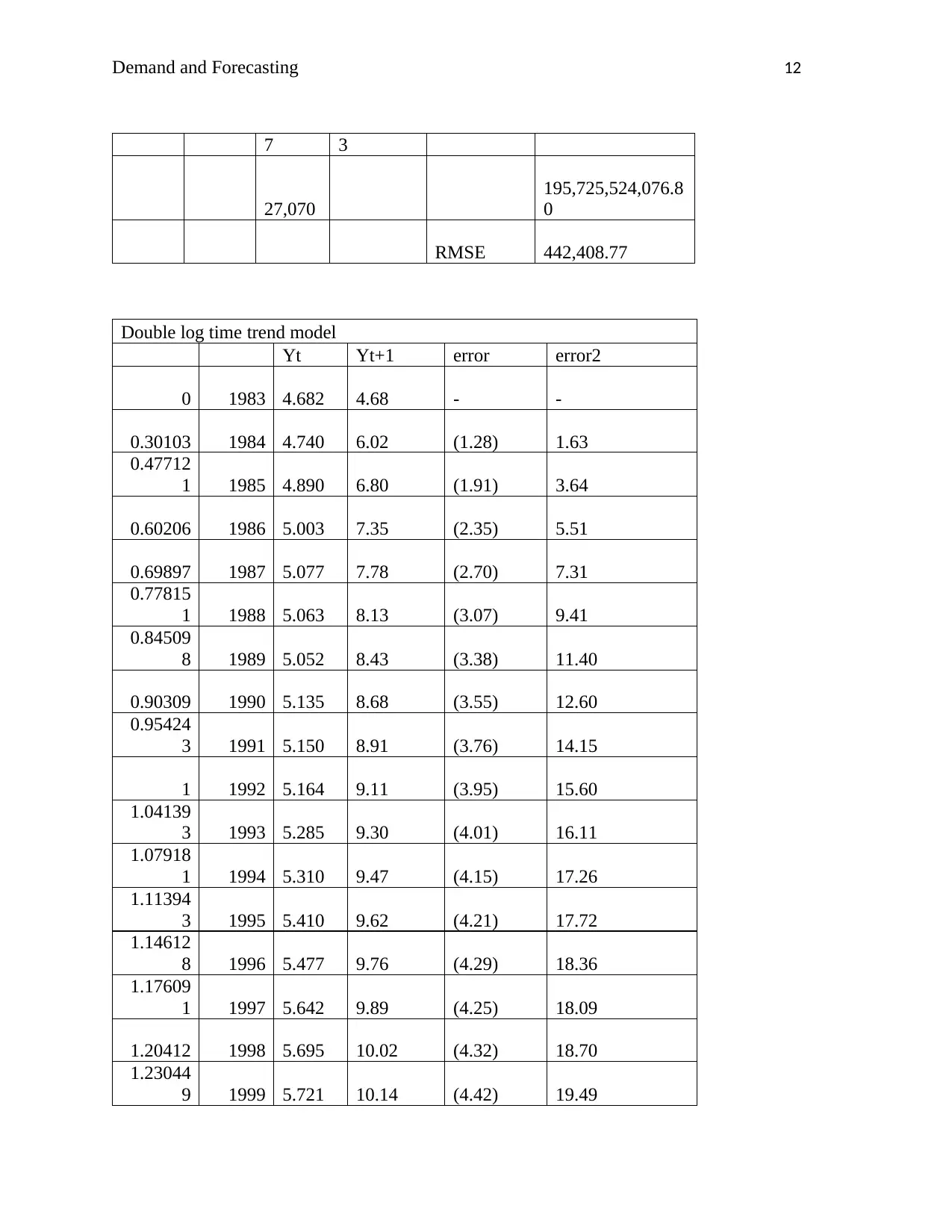
6. Estimate the double-log (log-linear) time trend model for log cruise ship arrivals
against log time. Estimate a linear time trend model of cruise ship arrivals against
time. Calculate the root mean square error between the predicted and actual value
of cruise ship arrivals. Is the root mean square error greater for the double log non-
linear time trend model or for the linear time trend model?
Linear time trend model
Yt Yt+1 error error2
1 1983 48,066 75,136.18 (27,070.18) 732,794,852.24
2 1984
54,907 102,206.3 (47,299.37) 2,237,230,179.81

Demand and Forecasting 11
7
3 1985 77,623
129,276.5
5 (51,653.55) 2,668,089,379.52
4 1986
100,69
5
156,346.7
4 (55,651.74) 3,097,115,641.25
5 1987
119,27
9
183,416.9
2 (64,137.92) 4,113,672,668.74
6 1988
115,50
5
210,487.1
0 (94,982.10) 9,021,599,879.13
7 1989
112,69
2
237,557.2
9
(124,865.29
) 15,591,339,838.83
8 1990
136,51
2
264,627.4
7
(128,115.47
) 16,413,573,804.05
9 1991
141,28
4
291,697.6
5
(150,413.65
) 22,624,267,433.50
10 1992
145,97
3
318,767.8
4
(172,794.84
) 29,858,056,120.76
11 1993
192,54
9
345,838.0
2
(153,289.02
) 23,497,524,283.75
12 1994
204,38
7
372,908.2
1
(168,521.21
) 28,399,396,832.04
13 1995
256,78
8
399,978.3
9
(143,190.39
) 20,503,487,704.12
14 1996
299,65
1
427,048.5
7
(127,397.57
) 16,230,141,741.18
15 1997
438,30
5
454,118.7
6 (15,813.76) 250,074,921.62
16 1998
494,96
1
481,188.9
4 13,772.06 189,669,604.24
17 1999
525,50 508,259.1 17,247.87 297,489,192.02

Demand and Forecasting 12
7 3
27,070
195,725,524,076.8
0
RMSE 442,408.77
Double log time trend model
Yt Yt+1 error error2
0 1983 4.682 4.68 - -
0.30103 1984 4.740 6.02 (1.28) 1.63
0.47712
1 1985 4.890 6.80 (1.91) 3.64
0.60206 1986 5.003 7.35 (2.35) 5.51
0.69897 1987 5.077 7.78 (2.70) 7.31
0.77815
1 1988 5.063 8.13 (3.07) 9.41
0.84509
8 1989 5.052 8.43 (3.38) 11.40
0.90309 1990 5.135 8.68 (3.55) 12.60
0.95424
3 1991 5.150 8.91 (3.76) 14.15
1 1992 5.164 9.11 (3.95) 15.60
1.04139
3 1993 5.285 9.30 (4.01) 16.11
1.07918
1 1994 5.310 9.47 (4.15) 17.26
1.11394
3 1995 5.410 9.62 (4.21) 17.72
1.14612
8 1996 5.477 9.76 (4.29) 18.36
1.17609
1 1997 5.642 9.89 (4.25) 18.09
1.20412 1998 5.695 10.02 (4.32) 18.70
1.23044
9 1999 5.721 10.14 (4.42) 19.49

Demand and Forecasting 13
4.432 206.99
14.39
It is evident that the root mean square is greater for a linear time trend compared to the log time
model.
Chapter 6
It can be seen that a decrease in the real interest rate in the United States results in a decrease in
the dollar. Consequently, it can also be seen that when the interest rate was highest in the United
States, the dollar was at its highest as seen in figure 6.1 and table 6.1 (McGuigan, Moyer, &
Harris, 2013). Thus, the dollar is poised to rise as the trend of the interest is on the rise.
A similar trend could also be seen for the growth rate. The growth rate is lowest between 2008
and 2009. Similar, during this period, the dollar is at its lowest between these two years. Thus,
with a positive outlook going into 2016, the dollar is poised to increase.
On the other hand, inflation has a positive relationship with the dollar (Jedrzejczyk, 2012). As
inflation decreases, the dollar also decreases and the opposite is true as seen in figure 6.1 and
table 6.1 (McGuigan, Moyer, & Harris, 2013). With the economy seen to entering into a negative
state of inflation going forward, then the dollar should be expected to lower in 2016.

Demand and Forecasting 14
Reference
Jedrzejczyk, M. (2012). Labor productivity parity vs trend of exchange rate. Modern
Economy, 3(06), 780.
McGuigan, J., Moyer, R. C., & Harris, F. (2013). Managerial economics: applications,
strategies and tactics. Nelson Education.