Statistical Analysis of Company Revenue and Employee Salaries
VerifiedAdded on 2019/11/20
|10
|1716
|326
Homework Assignment
AI Summary
This statistics assignment presents a comprehensive analysis of various statistical concepts. Question 1 focuses on descriptive statistics, constructing confidence intervals, and hypothesis testing related to company revenue. Question 2 explores hypothesis testing using proportions, analyzing the age of arsonists. Question 3 delves into comparing salaries, utilizing line graphs and t-tests to determine salary differences between genders, and calculating confidence intervals. Question 4 covers probability calculations using z-scores and the central limit theorem, including sampling distributions. Question 5 differentiates between parameters and statistics, explaining the law of large numbers and the central limit theorem. Finally, Question 6 investigates the impact of alcohol consumption on test scores using both a paired t-test and a non-parametric test (Spearman’s Rank Correlation), providing interpretations and conclusions for each analysis. The assignment demonstrates practical applications of statistical methods and their interpretations.
Question 1
a)
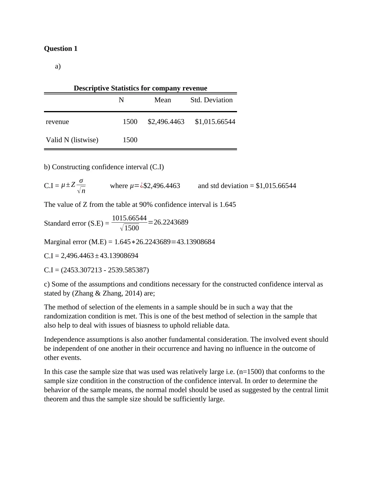
Descriptive Statistics for company revenue
N Mean Std. Deviation
revenue 1500 $2,496.4463 $1,015.66544
Valid N (listwise) 1500
b) Constructing confidence interval (C.I)
C.I = μ ± Z σ
√n where μ=¿$2,496.4463 and std deviation = $1,015.66544
The value of Z from the table at 90% confidence interval is 1.645
Standard error (S.E) = 1015.66544
√1500 =26.2243689
Marginal error (M.E) = 1.645∗26.2243689=43.13908684
C.I = 2,496.4463 ± 43.13908694
C.I = (2453.307213 - 2539.585387)
c) Some of the assumptions and conditions necessary for the constructed confidence interval as
stated by (Zhang & Zhang, 2014) are;
The method of selection of the elements in a sample should be in such a way that the
randomization condition is met. This is one of the best method of selection in the sample that
also help to deal with issues of biasness to uphold reliable data.
Independence assumptions is also another fundamental consideration. The involved event should
be independent of one another in their occurrence and having no influence in the outcome of
other events.
In this case the sample size that was used was relatively large i.e. (n=1500) that conforms to the
sample size condition in the construction of the confidence interval. In order to determine the
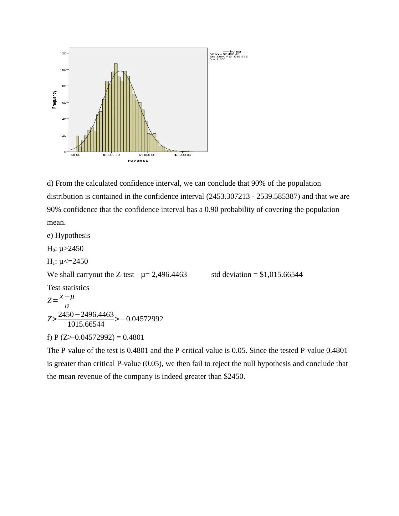
behavior of the sample means, the normal model should be used as suggested by the central limit
theorem and thus the sample size should be sufficiently large.
Paraphrase This Document
Need a fresh take? Get an instant paraphrase of this document with our AI Paraphraser
d) From the calculated confidence interval, we can conclude that 90% of the population
distribution is contained in the confidence interval (2453.307213 - 2539.585387) and that we are
90% confidence that the confidence interval has a 0.90 probability of covering the population
mean.
e) Hypothesis
H0: μ>2450
H1: μ<=2450
We shall carryout the Z-test μ= 2,496.4463 std deviation = $1,015.66544
Test statistics
Z= x −μ
σ
Z> 2450−2496.4463
1015.66544 >−0.04572992
f) P (Z>-0.04572992) = 0.4801
The P-value of the test is 0.4801 and the P-critical value is 0.05. Since the tested P-value 0.4801
is greater than critical P-value (0.05), we then fail to reject the null hypothesis and conclude that
the mean revenue of the company is indeed greater than $2450.
Question 2
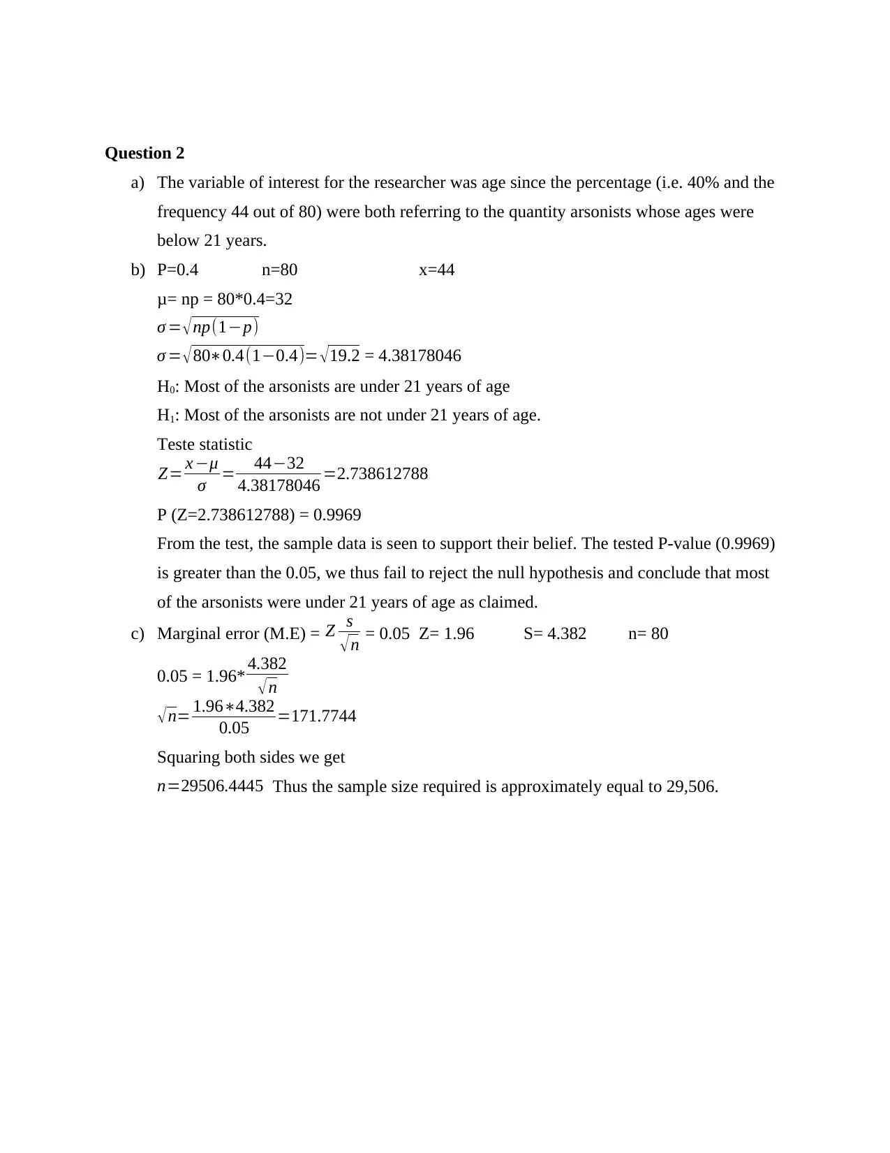
a) The variable of interest for the researcher was age since the percentage (i.e. 40% and the
frequency 44 out of 80) were both referring to the quantity arsonists whose ages were
below 21 years.
b) P=0.4 n=80 x=44
μ= np = 80*0.4=32
σ = √np(1−p)
σ = √ 80∗0.4(1−0.4)= √ 19.2 = 4.38178046
H0: Most of the arsonists are under 21 years of age
H1: Most of the arsonists are not under 21 years of age.
Teste statistic
Z= x −μ
σ = 44−32
4.38178046 =2.738612788
P (Z=2.738612788) = 0.9969
From the test, the sample data is seen to support their belief. The tested P-value (0.9969)
is greater than the 0.05, we thus fail to reject the null hypothesis and conclude that most
of the arsonists were under 21 years of age as claimed.
c) Marginal error (M.E) = Z s
√n = 0.05 Z= 1.96 S= 4.382 n= 80
0.05 = 1.96* 4.382
√n
√n= 1.96∗4.382
0.05 =171.7744
Squaring both sides we get
n=29506.4445 Thus the sample size required is approximately equal to 29,506.
⊘ This is a preview!⊘
Do you want full access?
Subscribe today to unlock all pages.

Trusted by 1+ million students worldwide
Question 3
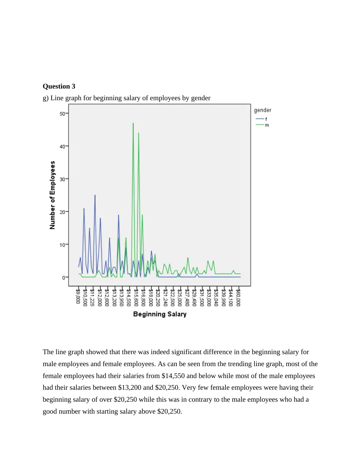
g) Line graph for beginning salary of employees by gender
The line graph showed that there was indeed significant difference in the beginning salary for
male employees and female employees. As can be seen from the trending line graph, most of the
female employees had their salaries from $14,550 and below while most of the male employees
had their salaries between $13,200 and $20,250. Very few female employees were having their
beginning salary of over $20,250 while this was in contrary to the male employees who had a
good number with starting salary above $20,250.
Paraphrase This Document
Need a fresh take? Get an instant paraphrase of this document with our AI Paraphraser
h) Hypothesis
H0: The mean for male beginning salary is not significantly greater than that of female
employees
H1: The mean for male beginning salary is significantly greater than that of the female employees
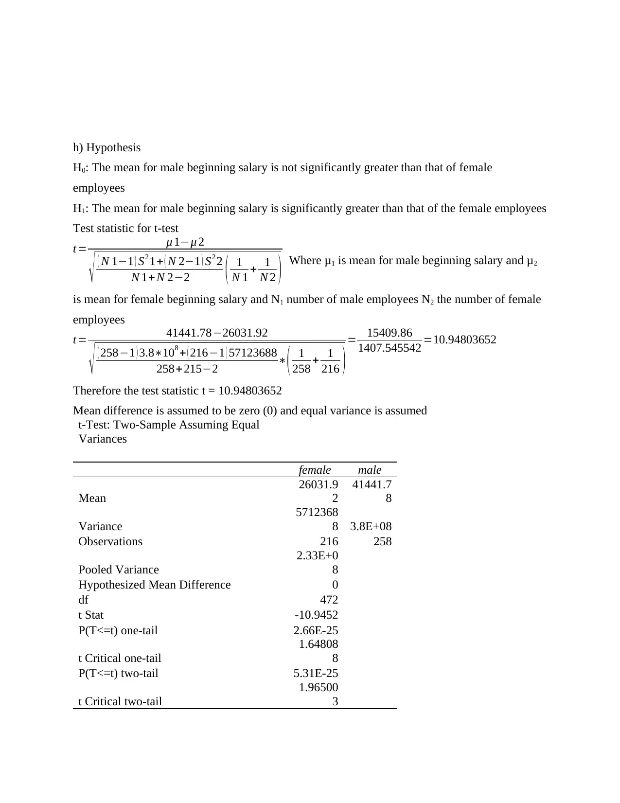
Test statistic for t-test
t= μ 1−μ 2
√ ( N 1−1 ) S2 1+ ( N 2−1 ) S2 2
N 1+ N 2−2 ( 1
N 1 + 1
N 2 ) Where μ1 is mean for male beginning salary and μ2
is mean for female beginning salary and N1 number of male employees N2 the number of female
employees
t= 41441.78−26031.92
√ ( 258−1 ) 3.8∗108 + ( 216−1 ) 57123688
258+ 215−2 ∗( 1
258 + 1
216 ) = 15409.86
1407.545542 =10.94803652
Therefore the test statistic t = 10.94803652
Mean difference is assumed to be zero (0) and equal variance is assumed
t-Test: Two-Sample Assuming Equal
Variances
female male
Mean
26031.9
2
41441.7
8
Variance
5712368
8 3.8E+08
Observations 216 258
Pooled Variance
2.33E+0
8
Hypothesized Mean Difference 0
df 472
t Stat -10.9452
P(T<=t) one-tail 2.66E-25
t Critical one-tail
1.64808
8
P(T<=t) two-tail 5.31E-25
t Critical two-tail
1.96500
3
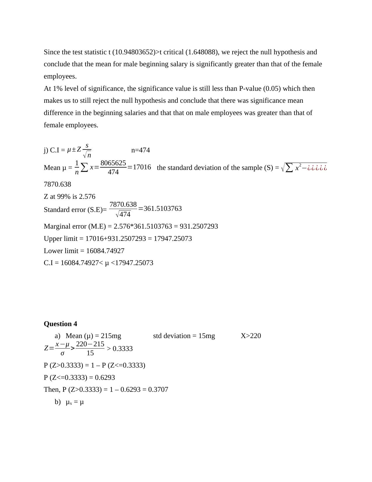
Since the test statistic t (10.94803652)>t critical (1.648088), we reject the null hypothesis and
conclude that the mean for male beginning salary is significantly greater than that of the female
employees.
At 1% level of significance, the significance value is still less than P-value (0.05) which then
makes us to still reject the null hypothesis and conclude that there was significance mean
difference in the beginning salaries and that that on male employees was greater than that of
female employees.
j) C.I = μ ± Z s
√ n n=474
Mean μ = 1
n ∑ x= 8065625
474 =17016 the standard deviation of the sample (S) = √∑ x2−¿ ¿ ¿ ¿ ¿
7870.638
Z at 99% is 2.576
Standard error (S.E)= 7870.638
√ 474 =361.5103763
Marginal error (M.E) = 2.576*361.5103763 = 931.2507293
Upper limit = 17016+931.2507293 = 17947.25073
Lower limit = 16084.74927
C.I = 16084.74927< μ <17947.25073
Question 4
a) Mean (μ) = 215mg std deviation = 15mg X>220
Z= x −μ
σ > 220−215
15 > 0.3333
P (Z>0.3333) = 1 – P (Z<=0.3333)
P (Z<=0.3333) = 0.6293
Then, P (Z>0.3333) = 1 – 0.6293 = 0.3707
b) μx = μ
⊘ This is a preview!⊘
Do you want full access?
Subscribe today to unlock all pages.

Trusted by 1+ million students worldwide
Sampling distribution of the sample mean is created when various samples of the same
size are drawn from a population and the sample means of each sample calculated for the
distribution. I.e. number of samples 25/5 = 5 samples with normal distribution.
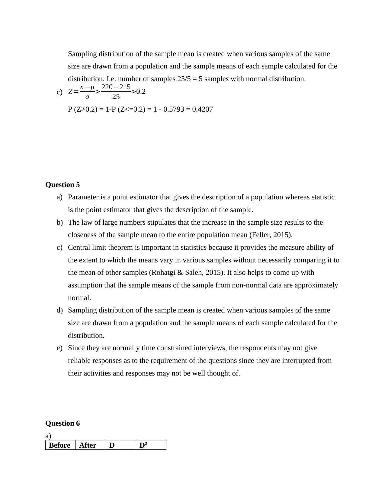
c) Z= x −μ
σ > 220−215
25 >0.2
P (Z>0.2) = 1-P (Z<=0.2) = 1 - 0.5793 = 0.4207
Question 5
a) Parameter is a point estimator that gives the description of a population whereas statistic
is the point estimator that gives the description of the sample.
b) The law of large numbers stipulates that the increase in the sample size results to the
closeness of the sample mean to the entire population mean (Feller, 2015).
c) Central limit theorem is important in statistics because it provides the measure ability of
the extent to which the means vary in various samples without necessarily comparing it to
the mean of other samples (Rohatgi & Saleh, 2015). It also helps to come up with
assumption that the sample means of the sample from non-normal data are approximately
normal.
d) Sampling distribution of the sample mean is created when various samples of the same
size are drawn from a population and the sample means of each sample calculated for the
distribution.
e) Since they are normally time constrained interviews, the respondents may not give
reliable responses as to the requirement of the questions since they are interrupted from
their activities and responses may not be well thought of.
Question 6
a)
Before After D D2
size are drawn from a population and the sample means of each sample calculated for the
distribution. I.e. number of samples 25/5 = 5 samples with normal distribution.
c) Z= x −μ
σ > 220−215
25 >0.2
P (Z>0.2) = 1-P (Z<=0.2) = 1 - 0.5793 = 0.4207
Question 5
a) Parameter is a point estimator that gives the description of a population whereas statistic
is the point estimator that gives the description of the sample.
b) The law of large numbers stipulates that the increase in the sample size results to the
closeness of the sample mean to the entire population mean (Feller, 2015).
c) Central limit theorem is important in statistics because it provides the measure ability of
the extent to which the means vary in various samples without necessarily comparing it to
the mean of other samples (Rohatgi & Saleh, 2015). It also helps to come up with
assumption that the sample means of the sample from non-normal data are approximately
normal.
d) Sampling distribution of the sample mean is created when various samples of the same
size are drawn from a population and the sample means of each sample calculated for the
distribution.
e) Since they are normally time constrained interviews, the respondents may not give
reliable responses as to the requirement of the questions since they are interrupted from
their activities and responses may not be well thought of.
Question 6
a)
Before After D D2
Paraphrase This Document
Need a fresh take? Get an instant paraphrase of this document with our AI Paraphraser
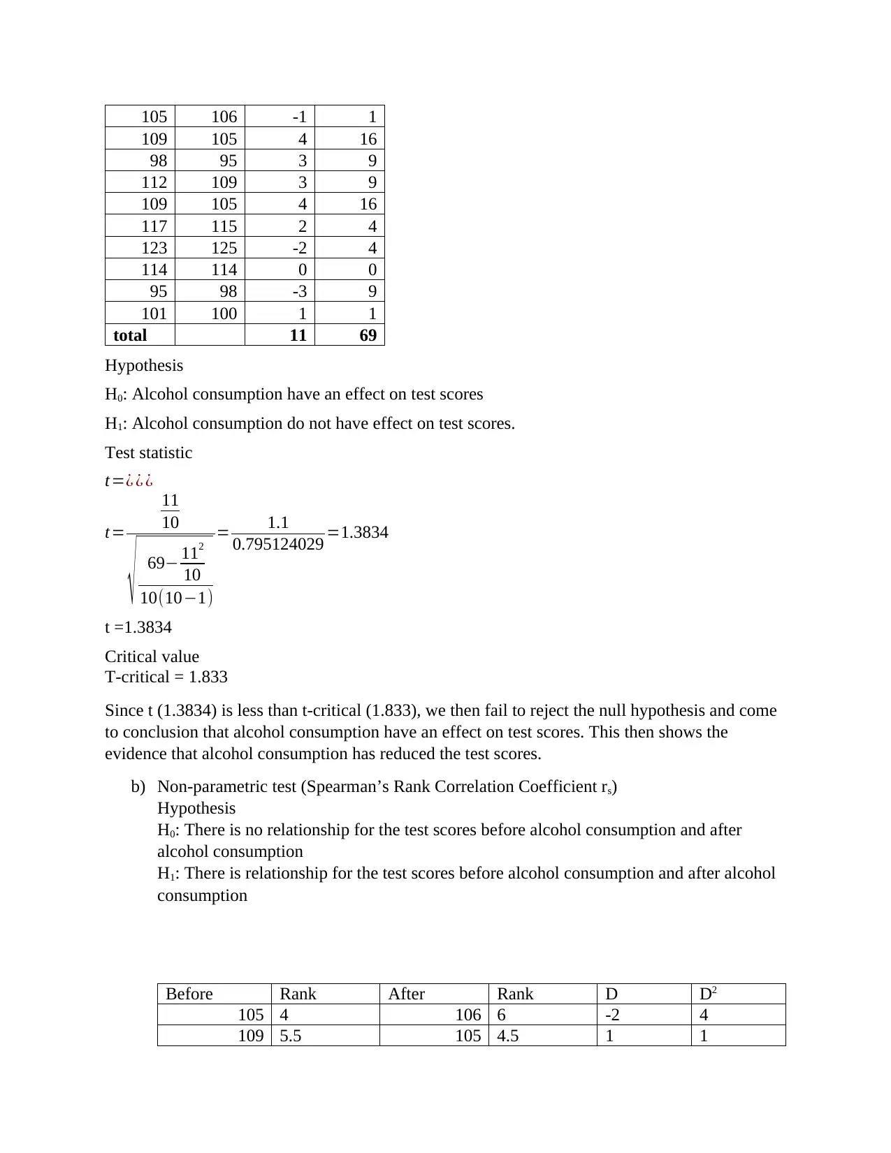
105 106 -1 1
109 105 4 16
98 95 3 9
112 109 3 9
109 105 4 16
117 115 2 4
123 125 -2 4
114 114 0 0
95 98 -3 9
101 100 1 1
total 11 69
Hypothesis
H0: Alcohol consumption have an effect on test scores
H1: Alcohol consumption do not have effect on test scores.
Test statistic
t=¿ ¿ ¿
t=
11
10
√ 69− 112
10
10(10−1)
= 1.1
0.795124029 =1.3834
t =1.3834
Critical value
T-critical = 1.833
Since t (1.3834) is less than t-critical (1.833), we then fail to reject the null hypothesis and come
to conclusion that alcohol consumption have an effect on test scores. This then shows the
evidence that alcohol consumption has reduced the test scores.
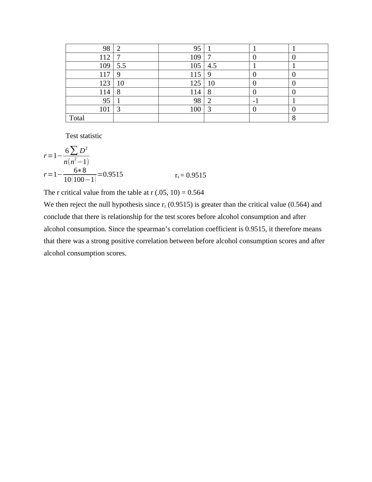
b) Non-parametric test (Spearman’s Rank Correlation Coefficient rs)
Hypothesis
H0: There is no relationship for the test scores before alcohol consumption and after
alcohol consumption
H1: There is relationship for the test scores before alcohol consumption and after alcohol
consumption
Before Rank After Rank D D2
105 4 106 6 -2 4
109 5.5 105 4.5 1 1
109 105 4 16
98 95 3 9
112 109 3 9
109 105 4 16
117 115 2 4
123 125 -2 4
114 114 0 0
95 98 -3 9
101 100 1 1
total 11 69
Hypothesis
H0: Alcohol consumption have an effect on test scores
H1: Alcohol consumption do not have effect on test scores.
Test statistic
t=¿ ¿ ¿
t=
11
10
√ 69− 112
10
10(10−1)
= 1.1
0.795124029 =1.3834
t =1.3834
Critical value
T-critical = 1.833
Since t (1.3834) is less than t-critical (1.833), we then fail to reject the null hypothesis and come
to conclusion that alcohol consumption have an effect on test scores. This then shows the
evidence that alcohol consumption has reduced the test scores.
b) Non-parametric test (Spearman’s Rank Correlation Coefficient rs)
Hypothesis
H0: There is no relationship for the test scores before alcohol consumption and after
alcohol consumption
H1: There is relationship for the test scores before alcohol consumption and after alcohol
consumption
Before Rank After Rank D D2
105 4 106 6 -2 4
109 5.5 105 4.5 1 1
98 2 95 1 1 1
112 7 109 7 0 0
109 5.5 105 4.5 1 1
117 9 115 9 0 0
123 10 125 10 0 0
114 8 114 8 0 0
95 1 98 2 -1 1
101 3 100 3 0 0
Total 8
Test statistic
r =1− 6 ∑ D2
n(n2 −1)
r =1− 6∗8
10 ( 100−1 ) =0.9515 rs = 0.9515
The r critical value from the table at r (.05, 10) = 0.564
We then reject the null hypothesis since rs (0.9515) is greater than the critical value (0.564) and
conclude that there is relationship for the test scores before alcohol consumption and after
alcohol consumption. Since the spearman’s correlation coefficient is 0.9515, it therefore means
that there was a strong positive correlation between before alcohol consumption scores and after
alcohol consumption scores.
⊘ This is a preview!⊘
Do you want full access?
Subscribe today to unlock all pages.

Trusted by 1+ million students worldwide
References
Feller, W. (2015). Note on the law of large numbers and “fair” games. In Selected Papers I (pp.
717-720). Springer International Publishing.
Rohatgi, V. K., & Saleh, A. M. E. (2015). An introduction to probability and statistics. John
Wiley & Sons.
Zhang, C. H., & Zhang, S. S. (2014). Confidence intervals for low dimensional parameters in
high dimensional linear models. Journal of the Royal Statistical Society: Series B
(Statistical Methodology), 76(1), 217-242.
1 out of 10
Related Documents
Your All-in-One AI-Powered Toolkit for Academic Success.
+13062052269
info@desklib.com
Available 24*7 on WhatsApp / Email
![[object Object]](/_next/static/media/star-bottom.7253800d.svg)
Unlock your academic potential
Copyright © 2020–2025 A2Z Services. All Rights Reserved. Developed and managed by ZUCOL.


