Desklib - Online Library for Study Material with Solved Assignments, Essays, Dissertations

Desklib is an online library for study material with solved assignments, essays, dissertations, and more. This article includes solved assignments for HI6007, ANOVA tables, regression analysis, and histograms. The article also includes information on the significance of variables and the impact of competitors' prices on weekly sales.

Running Head: HI6007: GROUP ASSIGNMENT
HI6007: Group Assignment
Name of the Student
Name of the University
Student ID

1HI6007: GROUP ASSIGNMENT
Table of Contents
Answer 1..........................................................................................................................................3
Part A...........................................................................................................................................3
Part B...........................................................................................................................................4
Answer 2..........................................................................................................................................5
Part A...........................................................................................................................................5
Part B...........................................................................................................................................5
Part C...........................................................................................................................................6
Part D...........................................................................................................................................6
Part E...........................................................................................................................................6
Answer 3..........................................................................................................................................7
Part A...........................................................................................................................................7
Part B...........................................................................................................................................7
Answer 4..........................................................................................................................................7
Part A...........................................................................................................................................7
Part B...........................................................................................................................................8
Part C...........................................................................................................................................9
Part D...........................................................................................................................................9
Part E.........................................................................................................................................10

2HI6007: GROUP ASSIGNMENT
Answer 1
Part A
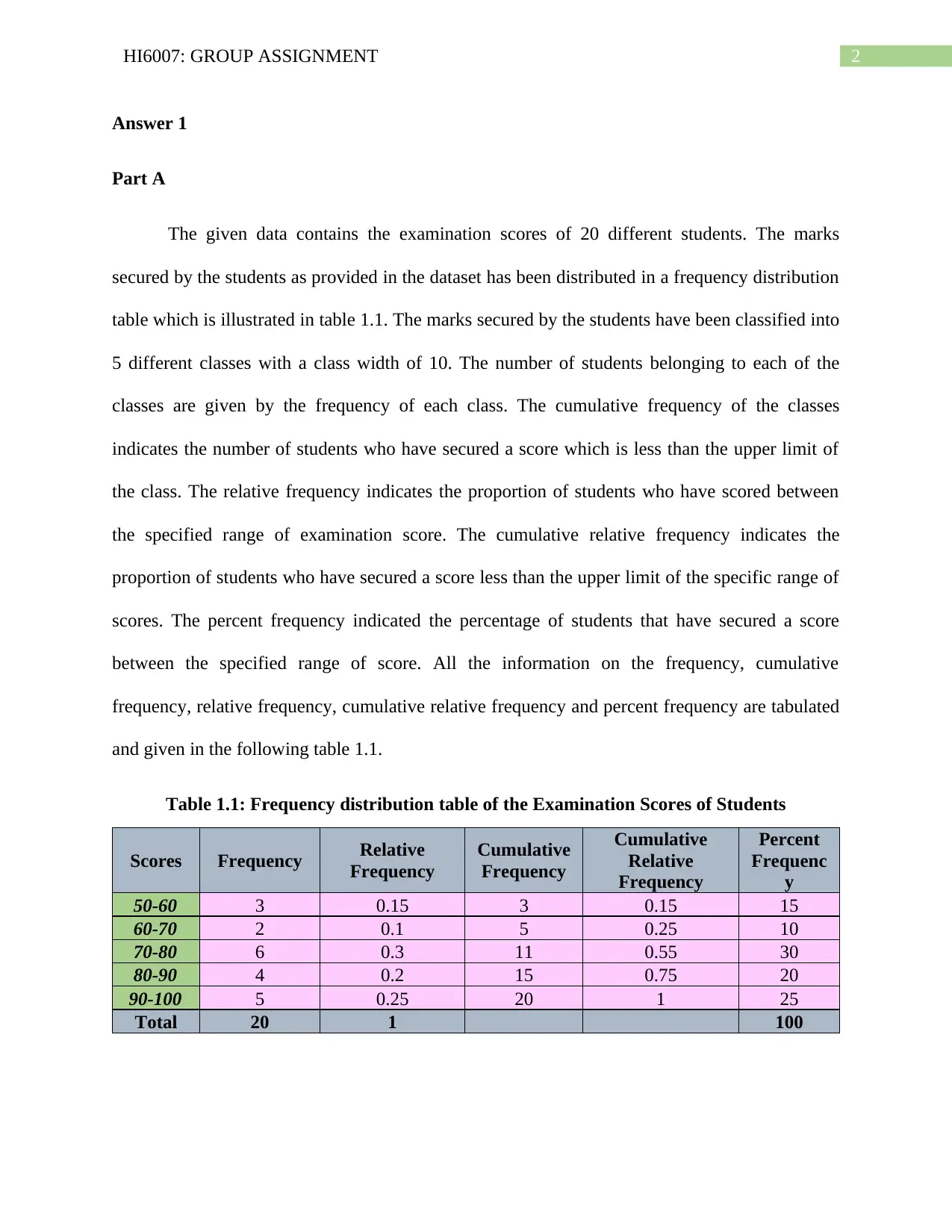
The given data contains the examination scores of 20 different students. The marks
secured by the students as provided in the dataset has been distributed in a frequency distribution
table which is illustrated in table 1.1. The marks secured by the students have been classified into
5 different classes with a class width of 10. The number of students belonging to each of the
classes are given by the frequency of each class. The cumulative frequency of the classes
indicates the number of students who have secured a score which is less than the upper limit of
the class. The relative frequency indicates the proportion of students who have scored between
the specified range of examination score. The cumulative relative frequency indicates the
proportion of students who have secured a score less than the upper limit of the specific range of
scores. The percent frequency indicated the percentage of students that have secured a score
between the specified range of score. All the information on the frequency, cumulative
frequency, relative frequency, cumulative relative frequency and percent frequency are tabulated
and given in the following table 1.1.
Table 1.1: Frequency distribution table of the Examination Scores of Students
Scores Frequency Relative
Frequency
Cumulative
Frequency
Cumulative
Relative
Frequency
Percent
Frequenc
y
50-60 3 0.15 3 0.15 15
60-70 2 0.1 5 0.25 10
70-80 6 0.3 11 0.55 30
80-90 4 0.2 15 0.75 20
90-100 5 0.25 20 1 25
Total 20 1 100

3HI6007: GROUP ASSIGNMENT
Part B
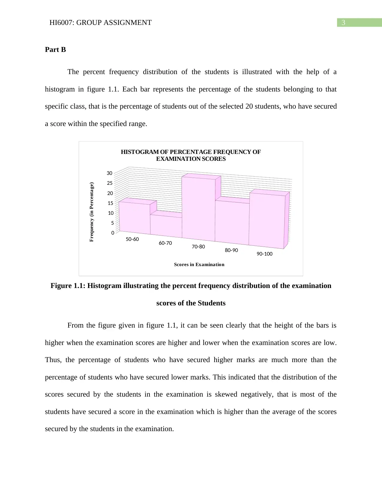
The percent frequency distribution of the students is illustrated with the help of a
histogram in figure 1.1. Each bar represents the percentage of the students belonging to that
specific class, that is the percentage of students out of the selected 20 students, who have secured
a score within the specified range.
50-60 60-70 70-80 80-90 90-100
0
5
10
15
20
25
30
HISTOGRAM OF PERCENTAGE FREQUENCY OF
EXAMINATION SCORES
Scores in Examination
Frequency (in Percentage)
Figure 1.1: Histogram illustrating the percent frequency distribution of the examination
scores of the Students
From the figure given in figure 1.1, it can be seen clearly that the height of the bars is
higher when the examination scores are higher and lower when the examination scores are low.
Thus, the percentage of students who have secured higher marks are much more than the
percentage of students who have secured lower marks. This indicated that the distribution of the
scores secured by the students in the examination is skewed negatively, that is most of the
students have secured a score in the examination which is higher than the average of the scores
secured by the students in the examination.

4HI6007: GROUP ASSIGNMENT
Answer 2
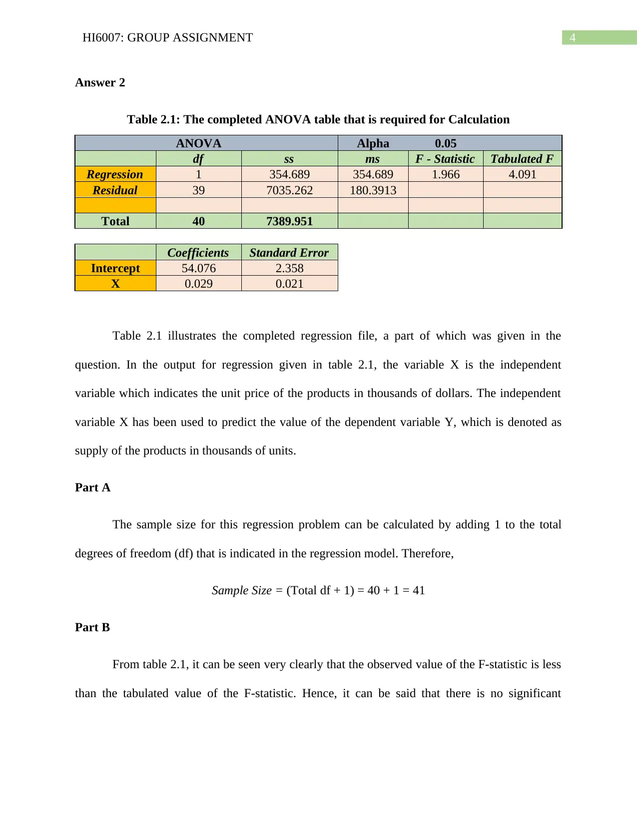
Table 2.1: The completed ANOVA table that is required for Calculation
ANOVA Alpha 0.05
df ss ms F - Statistic Tabulated F
Regression 1 354.689 354.689 1.966 4.091
Residual 39 7035.262 180.3913
Total 40 7389.951
Coefficients Standard Error
Intercept 54.076 2.358
X 0.029 0.021
Table 2.1 illustrates the completed regression file, a part of which was given in the
question. In the output for regression given in table 2.1, the variable X is the independent
variable which indicates the unit price of the products in thousands of dollars. The independent
variable X has been used to predict the value of the dependent variable Y, which is denoted as
supply of the products in thousands of units.
Part A
The sample size for this regression problem can be calculated by adding 1 to the total
degrees of freedom (df) that is indicated in the regression model. Therefore,
Sample Size = (Total df + 1) = 40 + 1 = 41
Part B
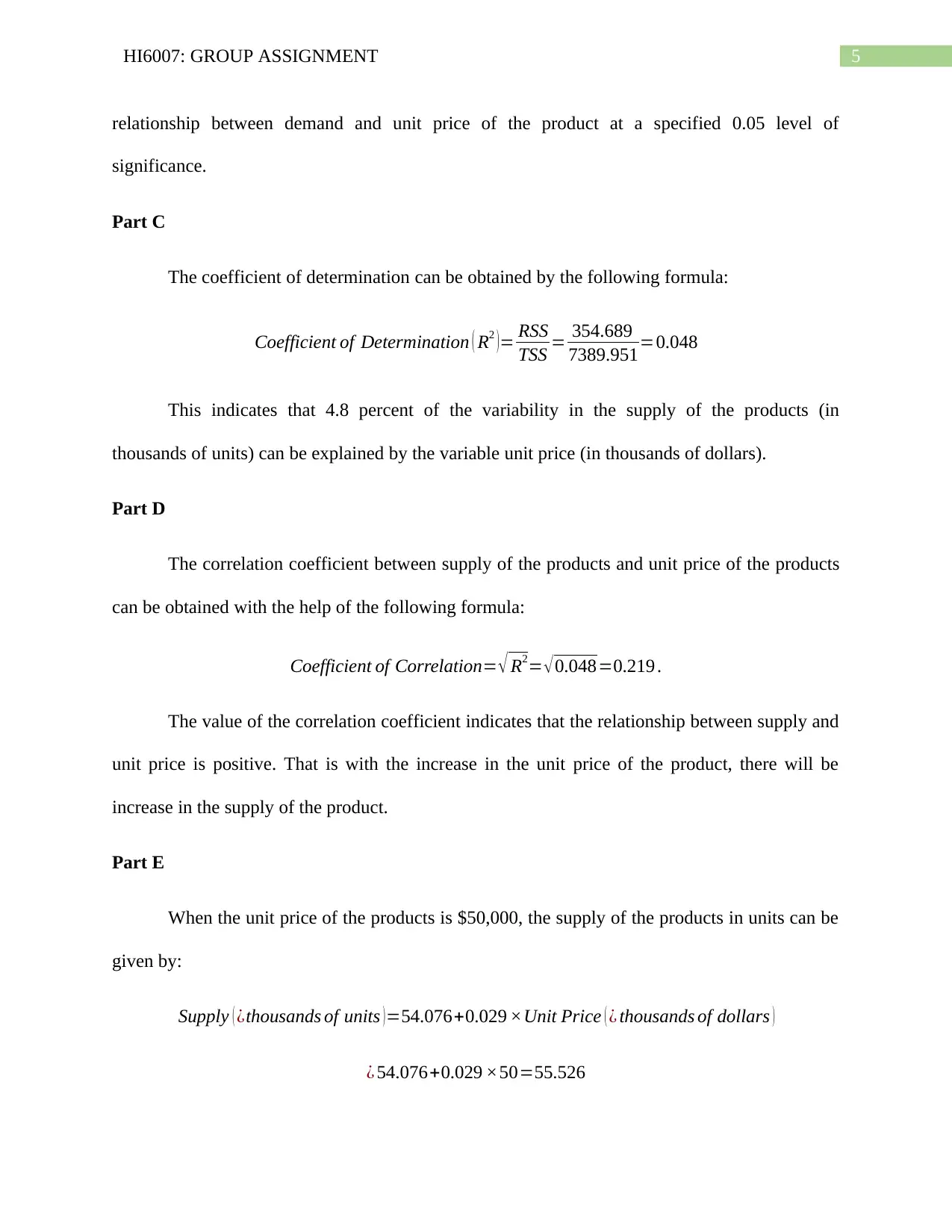
From table 2.1, it can be seen very clearly that the observed value of the F-statistic is less
than the tabulated value of the F-statistic. Hence, it can be said that there is no significant

5HI6007: GROUP ASSIGNMENT
relationship between demand and unit price of the product at a specified 0.05 level of
significance.
Part C
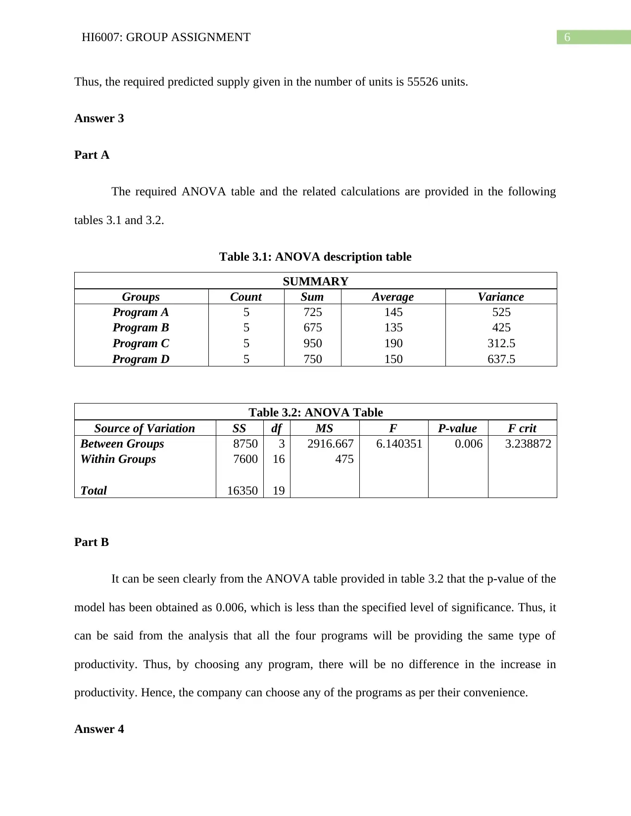
The coefficient of determination can be obtained by the following formula:
Coefficient of Determination ( R2 )= RSS
TSS = 354.689
7389.951=0.048
This indicates that 4.8 percent of the variability in the supply of the products (in
thousands of units) can be explained by the variable unit price (in thousands of dollars).
Part D
The correlation coefficient between supply of the products and unit price of the products
can be obtained with the help of the following formula:
Coefficient of Correlation= √ R2= √0.048=0.219 .
The value of the correlation coefficient indicates that the relationship between supply and
unit price is positive. That is with the increase in the unit price of the product, there will be
increase in the supply of the product.
Part E
When the unit price of the products is $50,000, the supply of the products in units can be
given by:
Supply ( ¿thousands of units )=54.076+0.029 ×Unit Price ( ¿ thousands of dollars )
¿ 54.076+0.029 ×50=55.526

6HI6007: GROUP ASSIGNMENT
Thus, the required predicted supply given in the number of units is 55526 units.
Answer 3
Part A
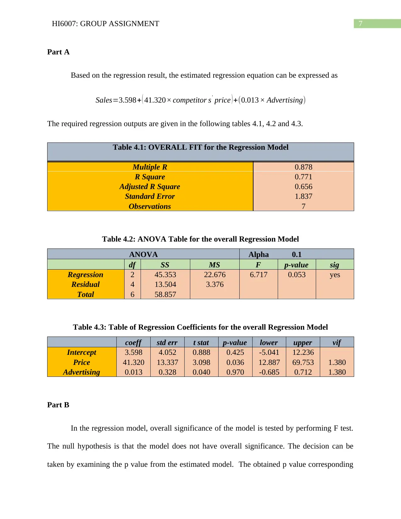
The required ANOVA table and the related calculations are provided in the following
tables 3.1 and 3.2.
Table 3.1: ANOVA description table
SUMMARY
Groups Count Sum Average Variance
Program A 5 725 145 525
Program B 5 675 135 425
Program C 5 950 190 312.5
Program D 5 750 150 637.5
Table 3.2: ANOVA Table
Source of Variation SS df MS F P-value F crit
Between Groups 8750 3 2916.667 6.140351 0.006 3.238872
Within Groups 7600 16 475
Total 16350 19
Part B
It can be seen clearly from the ANOVA table provided in table 3.2 that the p-value of the
model has been obtained as 0.006, which is less than the specified level of significance. Thus, it
can be said from the analysis that all the four programs will be providing the same type of
productivity. Thus, by choosing any program, there will be no difference in the increase in
productivity. Hence, the company can choose any of the programs as per their convenience.
Answer 4

7HI6007: GROUP ASSIGNMENT
Part A
Based on the regression result, the estimated regression equation can be expressed as
Sales=3.598+ ( 41.320× competitor s' price ) +(0.013 × Advertising)
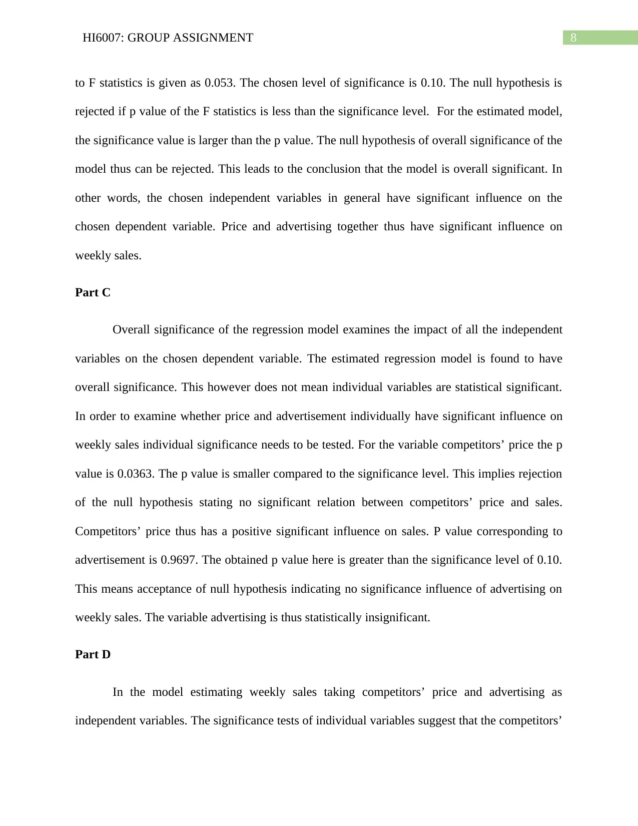
The required regression outputs are given in the following tables 4.1, 4.2 and 4.3.
Table 4.1: OVERALL FIT for the Regression Model
Multiple R 0.878
R Square 0.771
Adjusted R Square 0.656
Standard Error 1.837
Observations 7
Table 4.2: ANOVA Table for the overall Regression Model
ANOVA Alpha 0.1
df SS MS F p-value sig
Regression 2 45.353 22.676 6.717 0.053 yes
Residual 4 13.504 3.376
Total 6 58.857
Table 4.3: Table of Regression Coefficients for the overall Regression Model
coeff std err t stat p-value lower upper vif
Intercept 3.598 4.052 0.888 0.425 -5.041 12.236
Price 41.320 13.337 3.098 0.036 12.887 69.753 1.380
Advertising 0.013 0.328 0.040 0.970 -0.685 0.712 1.380
Part B
In the regression model, overall significance of the model is tested by performing F test.
The null hypothesis is that the model does not have overall significance. The decision can be
taken by examining the p value from the estimated model. The obtained p value corresponding

8HI6007: GROUP ASSIGNMENT
to F statistics is given as 0.053. The chosen level of significance is 0.10. The null hypothesis is
rejected if p value of the F statistics is less than the significance level. For the estimated model,
the significance value is larger than the p value. The null hypothesis of overall significance of the
model thus can be rejected. This leads to the conclusion that the model is overall significant. In
other words, the chosen independent variables in general have significant influence on the
chosen dependent variable. Price and advertising together thus have significant influence on
weekly sales.
Part C
Overall significance of the regression model examines the impact of all the independent
variables on the chosen dependent variable. The estimated regression model is found to have
overall significance. This however does not mean individual variables are statistical significant.
In order to examine whether price and advertisement individually have significant influence on
weekly sales individual significance needs to be tested. For the variable competitors’ price the p
value is 0.0363. The p value is smaller compared to the significance level. This implies rejection
of the null hypothesis stating no significant relation between competitors’ price and sales.
Competitors’ price thus has a positive significant influence on sales. P value corresponding to
advertisement is 0.9697. The obtained p value here is greater than the significance level of 0.10.
This means acceptance of null hypothesis indicating no significance influence of advertising on
weekly sales. The variable advertising is thus statistically insignificant.
Part D
In the model estimating weekly sales taking competitors’ price and advertising as
independent variables. The significance tests of individual variables suggest that the competitors’

9HI6007: GROUP ASSIGNMENT
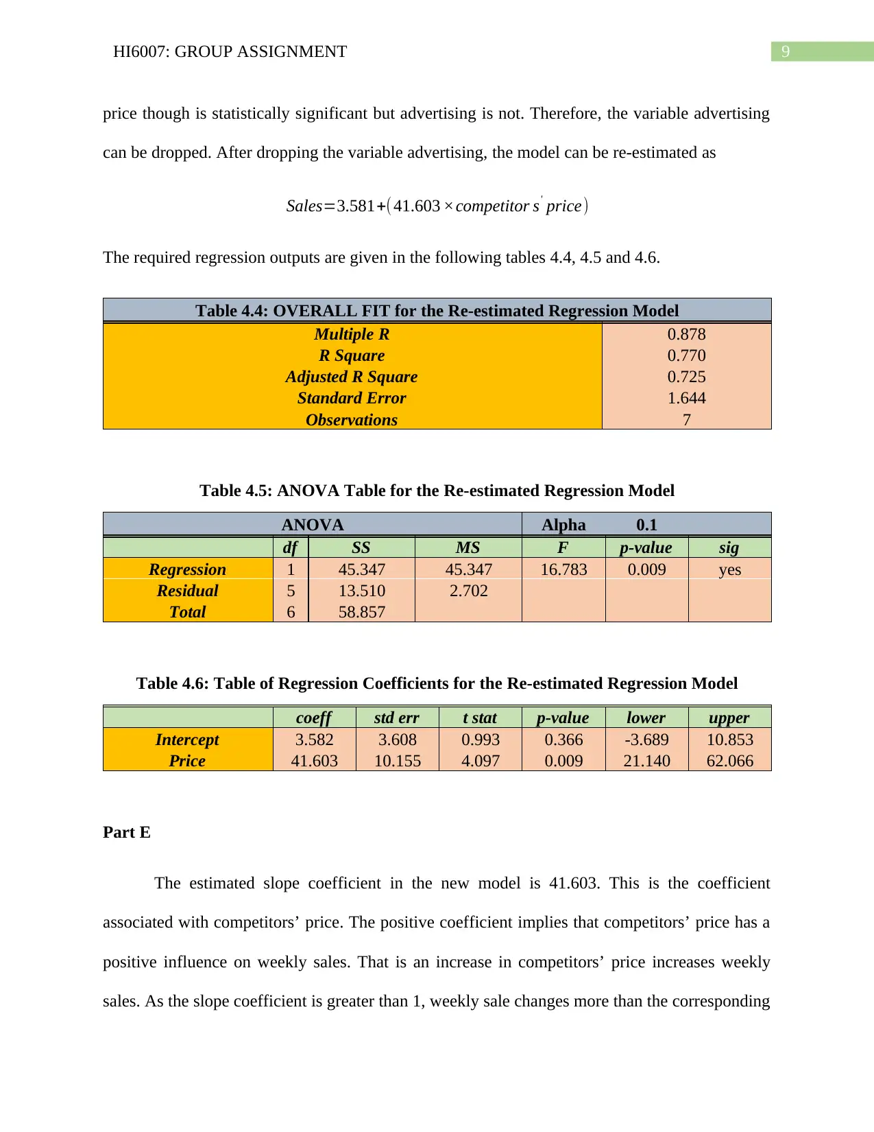
price though is statistically significant but advertising is not. Therefore, the variable advertising
can be dropped. After dropping the variable advertising, the model can be re-estimated as
Sales=3.581+( 41.603 ×competitor s' price)
The required regression outputs are given in the following tables 4.4, 4.5 and 4.6.
Table 4.4: OVERALL FIT for the Re-estimated Regression Model
Multiple R 0.878
R Square 0.770
Adjusted R Square 0.725
Standard Error 1.644
Observations 7
Table 4.5: ANOVA Table for the Re-estimated Regression Model
ANOVA Alpha 0.1
df SS MS F p-value sig
Regression 1 45.347 45.347 16.783 0.009 yes
Residual 5 13.510 2.702
Total 6 58.857
Table 4.6: Table of Regression Coefficients for the Re-estimated Regression Model
coeff std err t stat p-value lower upper
Intercept 3.582 3.608 0.993 0.366 -3.689 10.853
Price 41.603 10.155 4.097 0.009 21.140 62.066
Part E
The estimated slope coefficient in the new model is 41.603. This is the coefficient
associated with competitors’ price. The positive coefficient implies that competitors’ price has a
positive influence on weekly sales. That is an increase in competitors’ price increases weekly
sales. As the slope coefficient is greater than 1, weekly sale changes more than the corresponding

10HI6007: GROUP ASSIGNMENT
change in competitors’ price. From the magnitude of the slope coefficient, it can be said that 1%
increase in competitors’ price increase weekly sales by 41.6%. The economic rationale behind
this is simple. As competitor of the company raises price of its product, buyers tend to reduce
demand for the concerned company’s product and look for cheaper alternatives. This in turn
increases demand and sales of other competitors’ product. This explains the relation between
competitors’ price and weekly sales in terms of the slope coefficient.