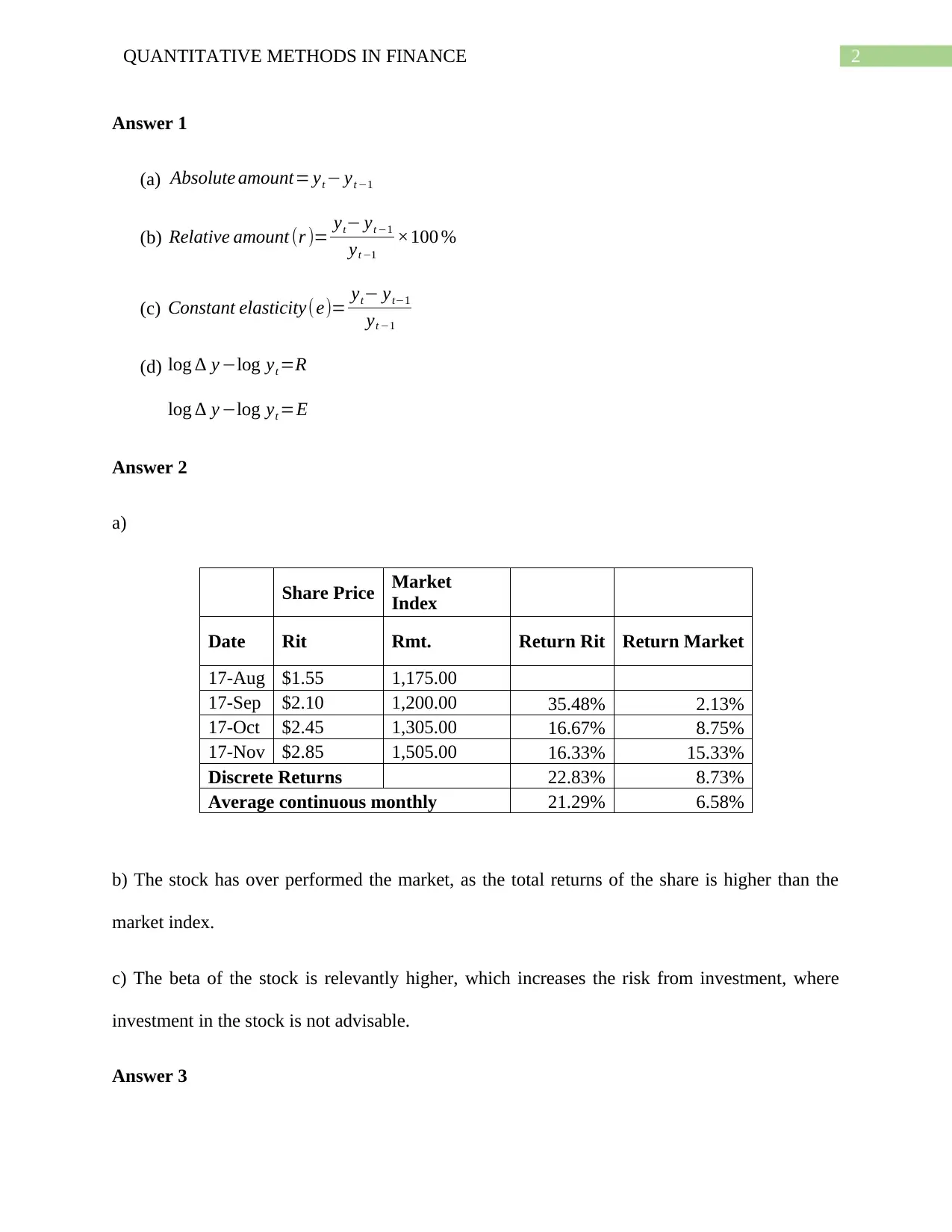
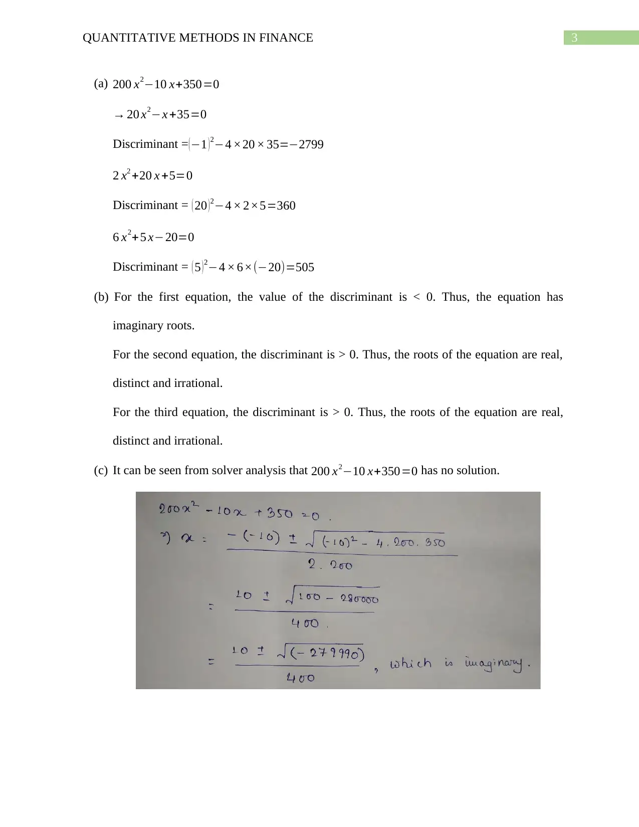
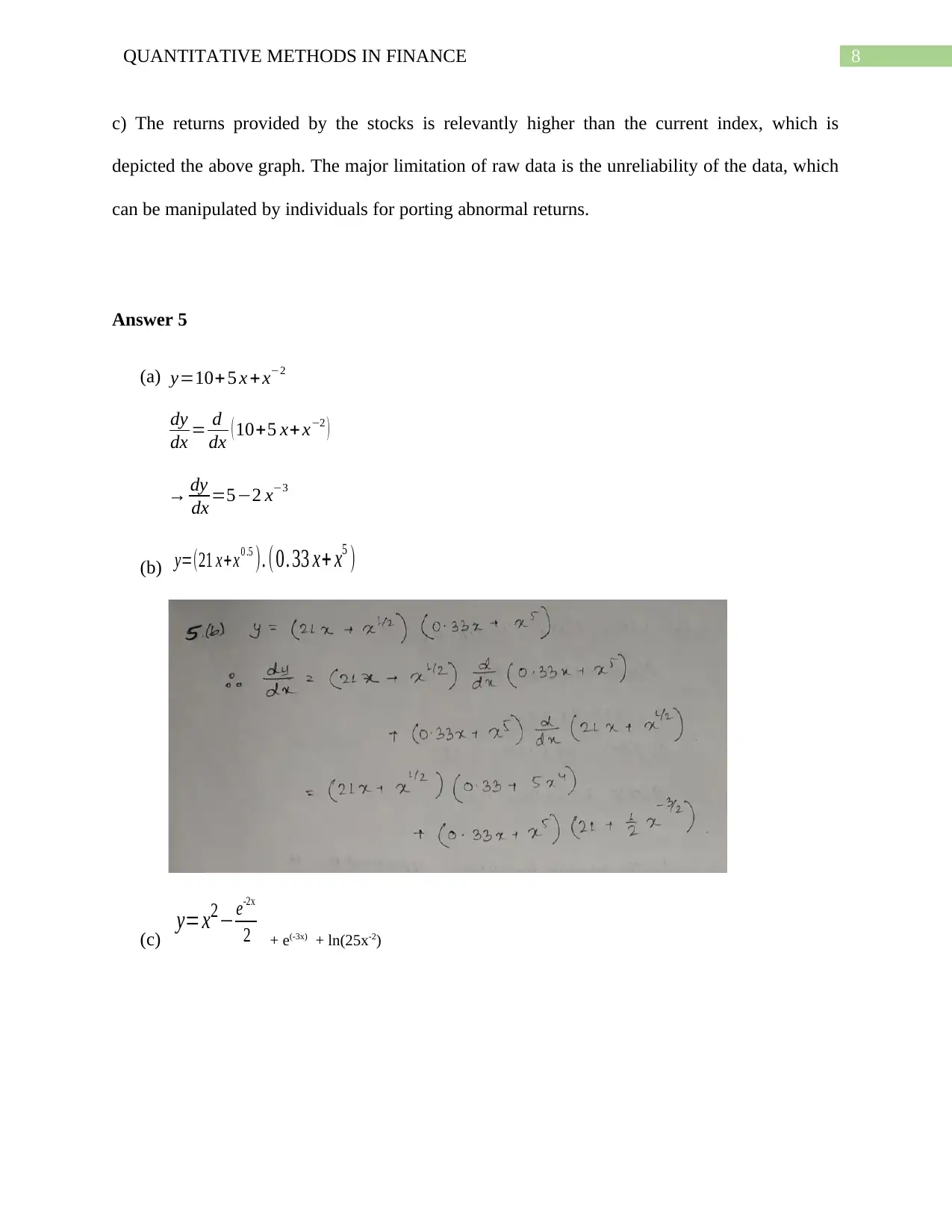
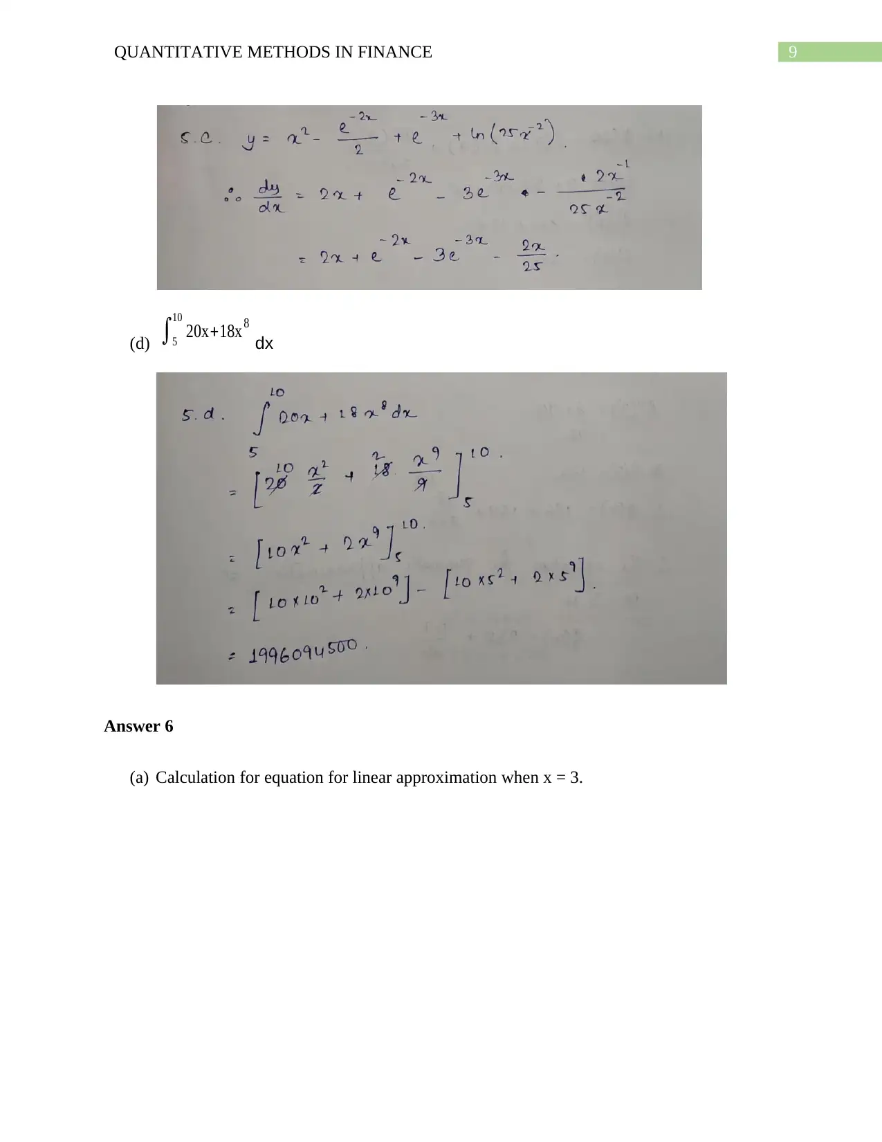
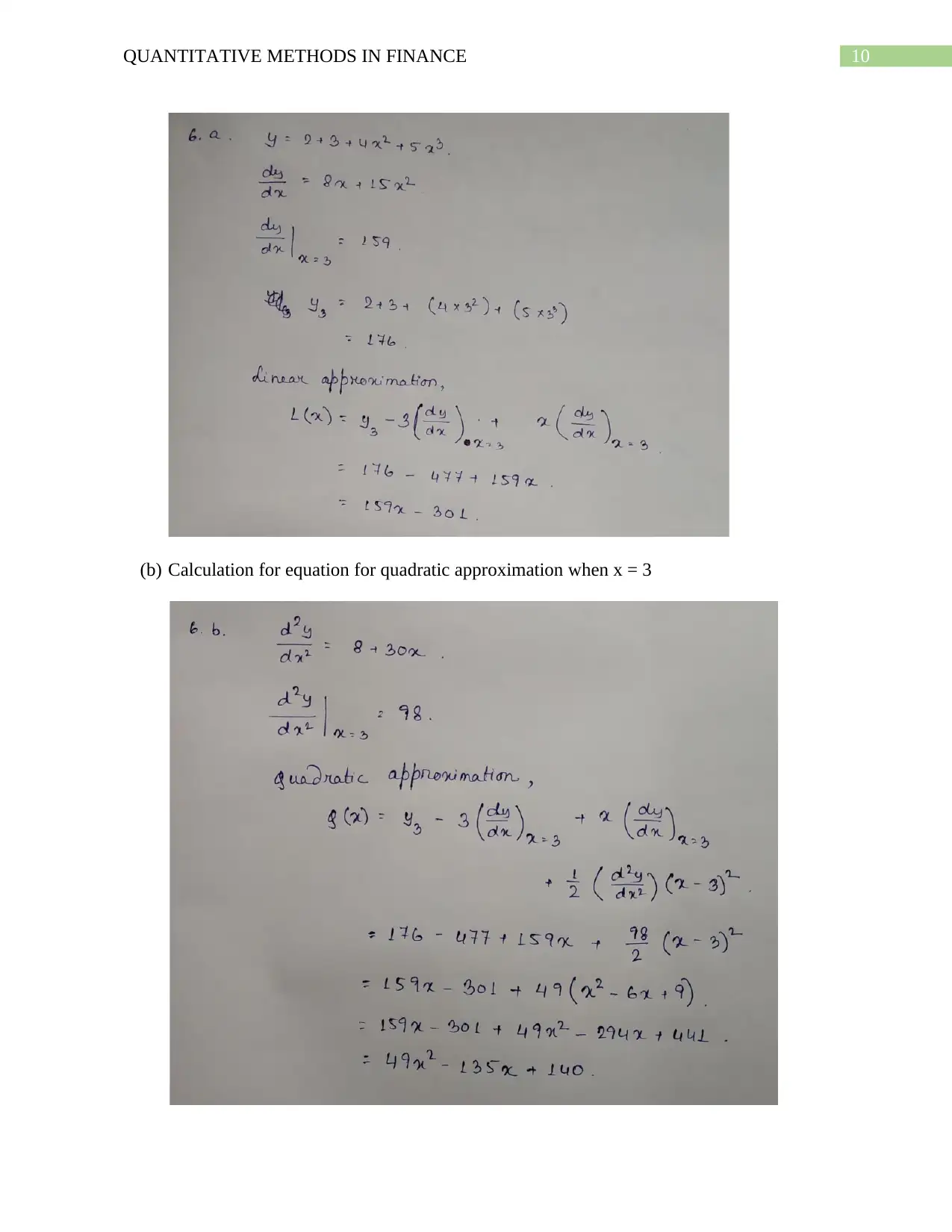
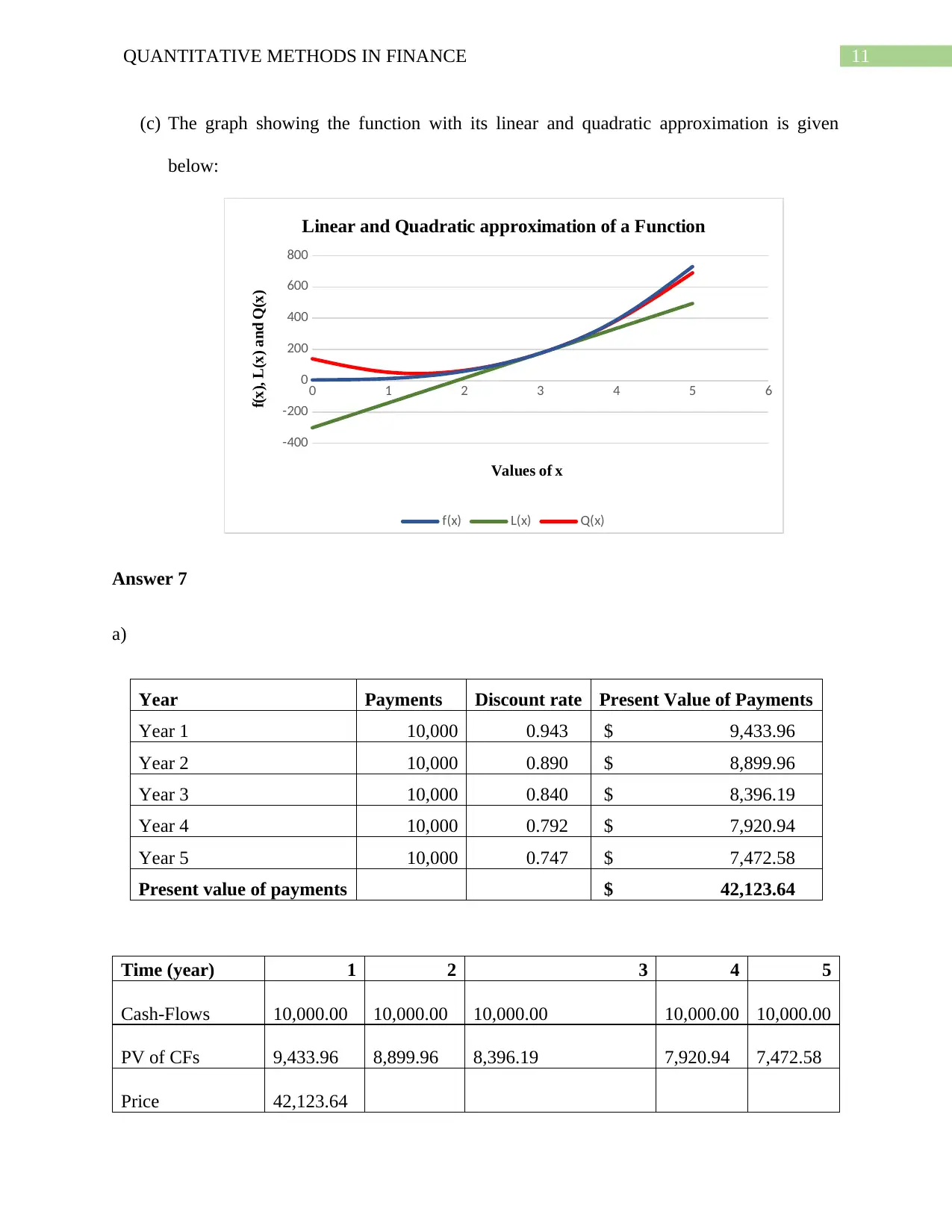
Desklib - Online Library for Study Material with Solved Assignments, Essays, Dissertation

This document covers various topics related to quantitative methods in finance, including quadratic equations, linear and quadratic approximations, bond valuation, and portfolio management. It also includes solved examples and graphs to help students understand the concepts better. The document is relevant for students pursuing finance courses in various universities and colleges.

Running Head: QUANTITATIVE METHODS IN FINANCE
Quantitative Methods in Finance
Name of the Student
Name of the University
Student ID

1QUANTITATIVE METHODS IN FINANCE
Table of Contents
Answer 1..........................................................................................................................................2
Answer 2..........................................................................................................................................2
Answer 3..........................................................................................................................................2
Answer 4..........................................................................................................................................7
Answer 5..........................................................................................................................................8
Answer 6..........................................................................................................................................9
Answer 7........................................................................................................................................11
Answer 8........................................................................................................................................12
Answer 9........................................................................................................................................13

2QUANTITATIVE METHODS IN FINANCE
Answer 1
(a) Absolute amount= yt − yt −1
(b) Relative amount (r )= yt− yt −1
yt −1
×100 %
(c) Constant elasticity(e)= yt− yt−1
yt −1
(d) log ∆ y −log yt =R
log ∆ y −log yt =E
Answer 2
a)
Share Price Market
Index
Date Rit Rmt. Return Rit Return Market
17-Aug $1.55 1,175.00
17-Sep $2.10 1,200.00 35.48% 2.13%
17-Oct $2.45 1,305.00 16.67% 8.75%
17-Nov $2.85 1,505.00 16.33% 15.33%
Discrete Returns 22.83% 8.73%
Average continuous monthly 21.29% 6.58%
b) The stock has over performed the market, as the total returns of the share is higher than the
market index.
c) The beta of the stock is relevantly higher, which increases the risk from investment, where
investment in the stock is not advisable.
Answer 3

3QUANTITATIVE METHODS IN FINANCE
(a) 200 x2−10 x+350=0
→ 20 x2−x +35=0
Discriminant =( −1 ) 2−4 ×20 × 35=−2799
2 x2 +20 x +5=0
Discriminant = ( 20 ) 2−4 × 2×5=360
6 x2+5 x−20=0
Discriminant = ( 5 ) 2−4 × 6×(−20)=505
(b) For the first equation, the value of the discriminant is < 0. Thus, the equation has
imaginary roots.
For the second equation, the discriminant is > 0. Thus, the roots of the equation are real,
distinct and irrational.
For the third equation, the discriminant is > 0. Thus, the roots of the equation are real,
distinct and irrational.
(c) It can be seen from solver analysis that 200 x2−10 x+350=0 has no solution.

4QUANTITATIVE METHODS IN FINANCE
The solution for the quadratic equation 2 x2 +20 x +5=0 is shown with the following
calculations:
The solutions for this quadratic as obtained from excel solver is shown in the following
figure:
The solution for the quadratic equation 6 x2+ 5 x−20=0 is shown with the following
calculations:

5QUANTITATIVE METHODS IN FINANCE
The solutions for this quadratic as obtained from excel solver is shown in the following
figure:
(d) The required graphs of the given equations are as follows:

6QUANTITATIVE METHODS IN FINANCE
0 2 4 6 8 10 12
0
5000
10000
15000
20000
25000
f(x) = 200x^2-10x+350
Value of x
f(x)
0 2 4 6 8 10 12
0
50
100
150
200
250
300
350
400
450
f(x) = 2x^2+20x+5
Value of x
f(x)

7QUANTITATIVE METHODS IN FINANCE
0 2 4 6 8 10 12
-100
0
100
200
300
400
500
600
700
f(x) = 6x^2+5x-20
Value of x
f(x)
Answer 4
a) answer in excel sheet
b)
7/7/2016
8/9/2016
9/11/2016
10/14/2016
11/16/2016
12/19/2016
1/21/2017
2/23/2017
3/28/2017
4/30/2017
6/2/2017
7/5/2017
8/7/2017
9/9/2017
10/12/2017
11/14/2017
12/17/2017
1/19/2018
2/21/2018
3/26/2018
4/28/2018
5/31/2018
7/3/2018
-200.00%
0.00%
200.00%
400.00%
600.00%
800.00%
1000.00%
Index S&P200 Index
Max Return LYNAS - UNADJUSTED PRICE
Min Return VOCUS GROUP - UNADJUSTED PRICE
Max Risk JANUS HENDERSON GROUP - UNADJUSTED PRICE

8QUANTITATIVE METHODS IN FINANCE
c) The returns provided by the stocks is relevantly higher than the current index, which is
depicted the above graph. The major limitation of raw data is the unreliability of the data, which
can be manipulated by individuals for porting abnormal returns.
Answer 5
(a) y=10+ 5 x +x−2
dy
dx = d
dx ( 10+5 x+ x−2 )
→ dy
dx =5−2 x−3
(b) y=(21 x+x0 .5 ). (0. 33 x+ x5 )
(c) y= x2− e-2x
2 + e(-3x) + ln(25x-2)

9QUANTITATIVE METHODS IN FINANCE
(d) ∫5
10
20x+18x8
dx
Answer 6
(a) Calculation for equation for linear approximation when x = 3.

10QUANTITATIVE METHODS IN FINANCE
(b) Calculation for equation for quadratic approximation when x = 3

11QUANTITATIVE METHODS IN FINANCE
(c) The graph showing the function with its linear and quadratic approximation is given
below:
0 1 2 3 4 5 6
-400
-200
0
200
400
600
800
Linear and Quadratic approximation of a Function
f(x) L(x) Q(x)
Values of x
f(x), L(x) and Q(x)
Answer 7
a)
Year Payments Discount rate Present Value of Payments
Year 1 10,000 0.943 $ 9,433.96
Year 2 10,000 0.890 $ 8,899.96
Year 3 10,000 0.840 $ 8,396.19
Year 4 10,000 0.792 $ 7,920.94
Year 5 10,000 0.747 $ 7,472.58
Present value of payments $ 42,123.64
Time (year) 1 2 3 4 5
Cash-Flows 10,000.00 10,000.00 10,000.00 10,000.00 10,000.00
PV of CFs 9,433.96 8,899.96 8,396.19 7,920.94 7,472.58
Price 42,123.64

12QUANTITATIVE METHODS IN FINANCE
Weighted CFs 10,000.00 20,000.00 30,000.00 40,000.00 50,000.00
PV of weighted
CFs 9,433.96 17,799.93 25,188.58 31,683.75 37,362.91
Sum of weight.
CFs
121,469.1
2
Duration 2.88
b)
Present value of payments $42,123.64
Duration 2.88
c)
Particulars Value
Portfolio value $ 8,219
Discount rate 6%
Time 5
Future value of Bond 5 years $46,331
Portfolio value $ 1,781
Discount rate 6%
Time 2
Future value of Bond 2 years $3,669
Total payments $50,000
Answer 8
BOND B1
Coupon
3.50
%

13QUANTITATIVE METHODS IN FINANCE
Face value 2000
Frequency 2
Maturity 2
Yield
6.00
%
Present Value of Price 1,907
Macaulay Dur 1.948
BOND B2
Coupon
4.50
%
Face value 2000
Frequency 2
Maturity 5
Yield
6.00
%
Present Value of Price 1,872
Macaulay Dur 4.514
BOND B3
Coupon
5.50
%
Face value 2000
Frequency 2
Maturity 10
Yield
6.00
%
Present Value of Price 1,926
Macaulay Dur 7.774
BOND B4
Coupon
6.50
%
Face value 2000
Frequency 2
Maturity 25
Yield
6.00
%

14QUANTITATIVE METHODS IN FINANCE
Present Value of Price 2,129
Macaulay Dur
13.04
1
Answer 9
a)
Particulars Value
Payment
$
20,000.00
Time 30
rate 3%
Present Value of the
payments $392,008.83
b)
Bond
s PV of contracts
Face
Value Total contracts Value
B1 1,907 2000 28 53,350.60
B2 1,872 2000 60 111,593.55
B3 1,926 2000 78 150,228.69
B4 2,129 2000 10 21,286.49
Cost of Establishing the
portfolio 336,459.33