Desklib - Online Library for Study Material with Solved Assignments, Essays, Dissertations

This document contains solutions to questions related to statistics and regression analysis. It discusses topics such as frequency tables, histograms, ANOVA, and regression equations. The content is relevant to students studying courses in statistics, mathematics, and data analysis in various colleges and universities.

Running head: HI6007 GROUP ASSIGNMENT
HI6007 GROUP ASSIGNMENT
Name of Student
Name of University
Author Note

1HI6007 GROUP ASSIGNMENT
Table of Contents
Question 1..................................................................................................................................2
Question 2..................................................................................................................................3
Question 3..................................................................................................................................4
Question 4..................................................................................................................................5

2HI6007 GROUP ASSIGNMENT
Question 1
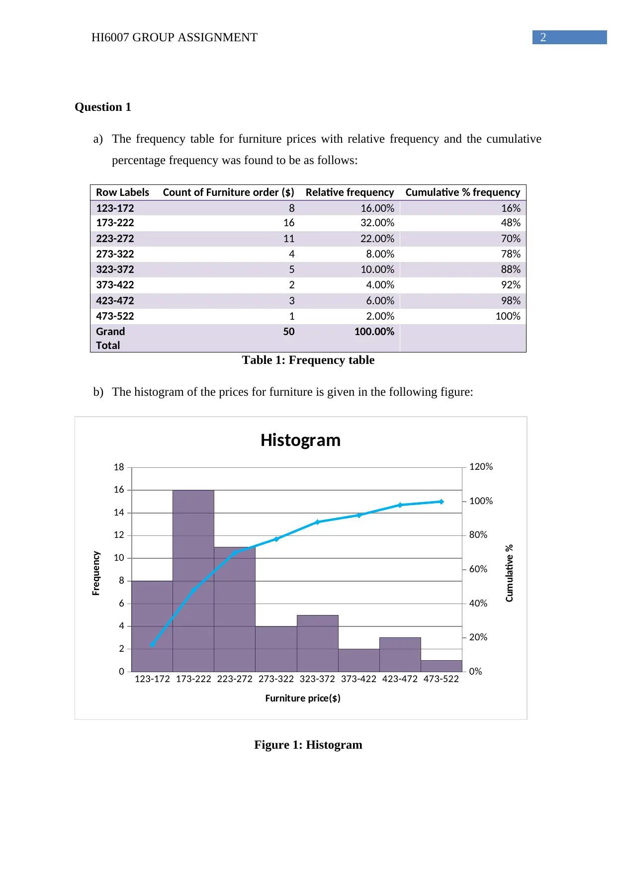
a) The frequency table for furniture prices with relative frequency and the cumulative
percentage frequency was found to be as follows:
Row Labels Count of Furniture order ($) Relative frequency Cumulative % frequency
123-172 8 16.00% 16%
173-222 16 32.00% 48%
223-272 11 22.00% 70%
273-322 4 8.00% 78%
323-372 5 10.00% 88%
373-422 2 4.00% 92%
423-472 3 6.00% 98%
473-522 1 2.00% 100%
Grand
Total
50 100.00%
Table 1: Frequency table
b) The histogram of the prices for furniture is given in the following figure:
123-172 173-222 223-272 273-322 323-372 373-422 423-472 473-522
0
2
4
6
8
10
12
14
16
18
0%
20%
40%
60%
80%
100%
120%
Histogram
Furniture price($)
Frequency
Cumulative %
Figure 1: Histogram

3HI6007 GROUP ASSIGNMENT
The histogram has a positively skewed shape with most of its frequency falling on the
left side. It has few high valued data whereas most of it is concentrated towards lower
amounts.
c) Due to presence of the few high values, falling above the 50% cumulative frequency
mark, the measure of average of the data would turn out to be higher than its real
measure of location. Thus a median would be a more appropriate metric for
measuring central tendency in this case.
Question 2
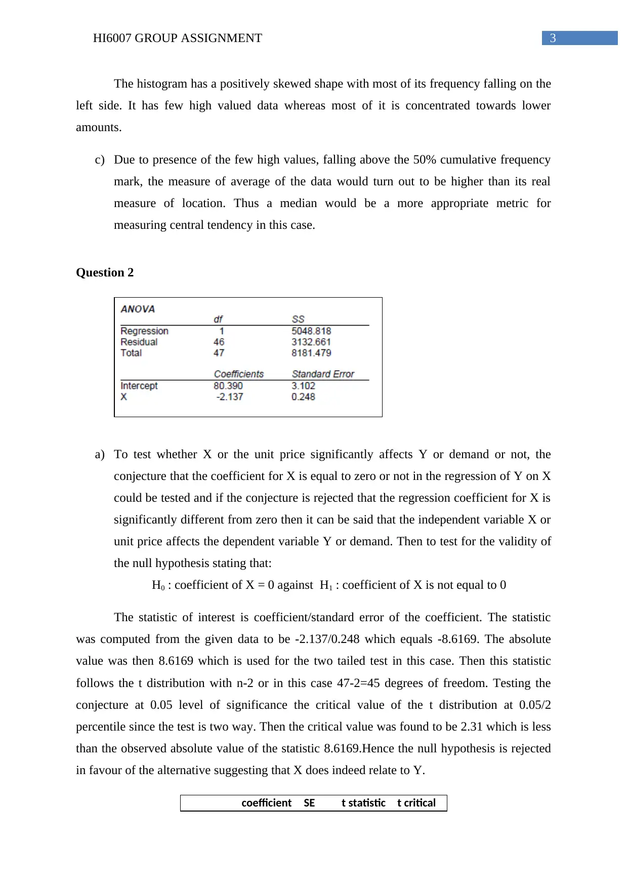
a) To test whether X or the unit price significantly affects Y or demand or not, the
conjecture that the coefficient for X is equal to zero or not in the regression of Y on X
could be tested and if the conjecture is rejected that the regression coefficient for X is
significantly different from zero then it can be said that the independent variable X or
unit price affects the dependent variable Y or demand. Then to test for the validity of
the null hypothesis stating that:
H0 : coefficient of X = 0 against H1 : coefficient of X is not equal to 0
The statistic of interest is coefficient/standard error of the coefficient. The statistic
was computed from the given data to be -2.137/0.248 which equals -8.6169. The absolute
value was then 8.6169 which is used for the two tailed test in this case. Then this statistic
follows the t distribution with n-2 or in this case 47-2=45 degrees of freedom. Testing the
conjecture at 0.05 level of significance the critical value of the t distribution at 0.05/2
percentile since the test is two way. Then the critical value was found to be 2.31 which is less
than the observed absolute value of the statistic 8.6169.Hence the null hypothesis is rejected
in favour of the alternative suggesting that X does indeed relate to Y.
coefficient SE t statistic t critical

4HI6007 GROUP ASSIGNMENT
intercep
t
80.39 3.102 25.91554
X -2.137 0.248 -8.61694 2.318891
Table 2: Summary specifications for Regression
b) The coefficient of determination is given by 1-(explained variance/total variance), that
is, 1-(sum of squares due to Regression model/ total sum of squares). It was thus
computed as 1-5048.818/8181.479, which equals 0.617103. This means that the
model that has been fitted here, which is Y on X explains 61.71% of the total
variation in the demand price, Y. It is a measure of how good the model fit the
observed data and is therefore used to gauge the goodness of fit of the model.
c) The correlation coefficient is the square root of the coefficient of determination and
was therefore computed to be 0.7855. It is a measure of the degree to which variation
in X affects the variation in Y and vice versa. The value here suggests that there is
moderate to high positive change in Y on the basis of X and vice versa. It is therefore
a measure of the association between the two variables.
Question 3
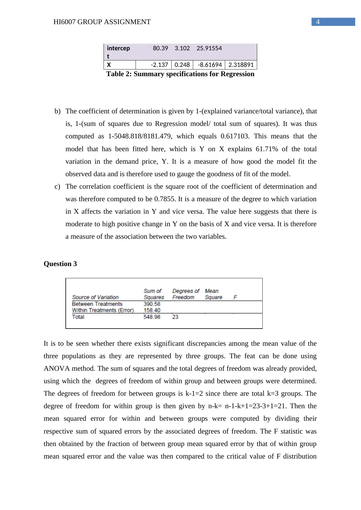
It is to be seen whether there exists significant discrepancies among the mean value of the
three populations as they are represented by three groups. The feat can be done using
ANOVA method. The sum of squares and the total degrees of freedom was already provided,
using which the degrees of freedom of within group and between groups were determined.
The degrees of freedom for between groups is k-1=2 since there are total k=3 groups. The
degree of freedom for within group is then given by n-k= n-1-k+1=23-3+1=21. Then the
mean squared error for within and between groups were computed by dividing their
respective sum of squared errors by the associated degrees of freedom. The F statistic was
then obtained by the fraction of between group mean squared error by that of within group
mean squared error and the value was then compared to the critical value of F distribution

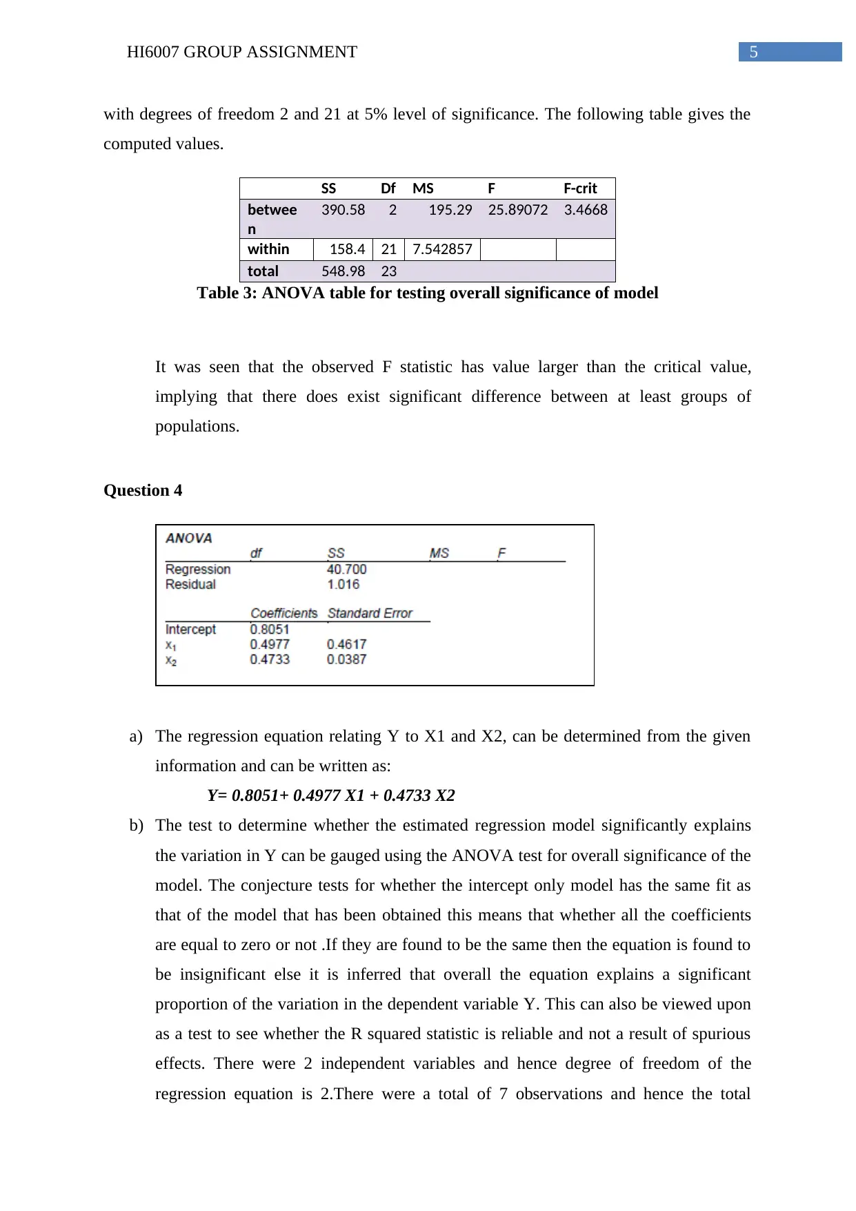
5HI6007 GROUP ASSIGNMENT
with degrees of freedom 2 and 21 at 5% level of significance. The following table gives the
computed values.
SS Df MS F F-crit
betwee
n
390.58 2 195.29 25.89072 3.4668
within 158.4 21 7.542857
total 548.98 23
Table 3: ANOVA table for testing overall significance of model
It was seen that the observed F statistic has value larger than the critical value,
implying that there does exist significant difference between at least groups of
populations.
Question 4
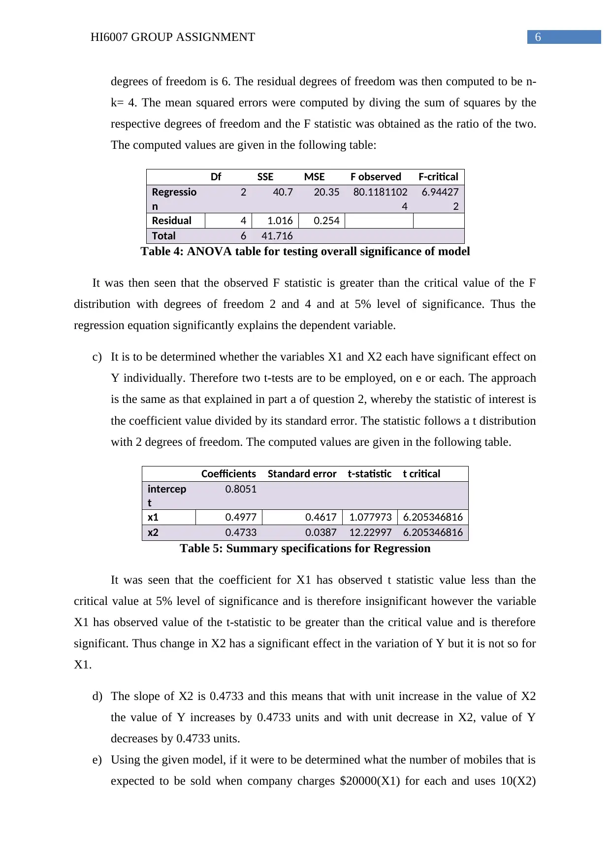
a) The regression equation relating Y to X1 and X2, can be determined from the given
information and can be written as:
Y= 0.8051+ 0.4977 X1 + 0.4733 X2
b) The test to determine whether the estimated regression model significantly explains
the variation in Y can be gauged using the ANOVA test for overall significance of the
model. The conjecture tests for whether the intercept only model has the same fit as
that of the model that has been obtained this means that whether all the coefficients
are equal to zero or not .If they are found to be the same then the equation is found to
be insignificant else it is inferred that overall the equation explains a significant
proportion of the variation in the dependent variable Y. This can also be viewed upon
as a test to see whether the R squared statistic is reliable and not a result of spurious
effects. There were 2 independent variables and hence degree of freedom of the
regression equation is 2.There were a total of 7 observations and hence the total

6HI6007 GROUP ASSIGNMENT
degrees of freedom is 6. The residual degrees of freedom was then computed to be n-
k= 4. The mean squared errors were computed by diving the sum of squares by the
respective degrees of freedom and the F statistic was obtained as the ratio of the two.
The computed values are given in the following table:
Df SSE MSE F observed F-critical
Regressio
n
2 40.7 20.35 80.1181102
4
6.94427
2
Residual 4 1.016 0.254
Total 6 41.716
Table 4: ANOVA table for testing overall significance of model
It was then seen that the observed F statistic is greater than the critical value of the F
distribution with degrees of freedom 2 and 4 and at 5% level of significance. Thus the
regression equation significantly explains the dependent variable.
c) It is to be determined whether the variables X1 and X2 each have significant effect on
Y individually. Therefore two t-tests are to be employed, on e or each. The approach
is the same as that explained in part a of question 2, whereby the statistic of interest is
the coefficient value divided by its standard error. The statistic follows a t distribution
with 2 degrees of freedom. The computed values are given in the following table.
Coefficients Standard error t-statistic t critical
intercep
t
0.8051
x1 0.4977 0.4617 1.077973 6.205346816
x2 0.4733 0.0387 12.22997 6.205346816
Table 5: Summary specifications for Regression
It was seen that the coefficient for X1 has observed t statistic value less than the
critical value at 5% level of significance and is therefore insignificant however the variable
X1 has observed value of the t-statistic to be greater than the critical value and is therefore
significant. Thus change in X2 has a significant effect in the variation of Y but it is not so for
X1.
d) The slope of X2 is 0.4733 and this means that with unit increase in the value of X2
the value of Y increases by 0.4733 units and with unit decrease in X2, value of Y
decreases by 0.4733 units.
e) Using the given model, if it were to be determined what the number of mobiles that is
expected to be sold when company charges $20000(X1) for each and uses 10(X2)

7HI6007 GROUP ASSIGNMENT
advertising spots, then plugging X1=$20,000 and X2=10, into th regression equation
specified in part a, it is found:
Y = 0.8051+ 0.4977 × 20000 + 0.4733× 10 = 9959.538 which is approximately 9959.
Hence as per the model 9959 units are sold given the specifications.