Desklib - Online Library for Study Material with Solved Assignments, Essays, Dissertations

Desklib is an online library for study material with solved assignments, essays, dissertations, and more. It offers a vast collection of study resources for various subjects and courses. The platform provides access to high-quality study material that can help students excel in their academics. Whether you are looking for solved assignments, essays, dissertations, or any other study material, Desklib has got you covered. The platform is suitable for students from different colleges and universities.

All your assignment looks correct expect the following
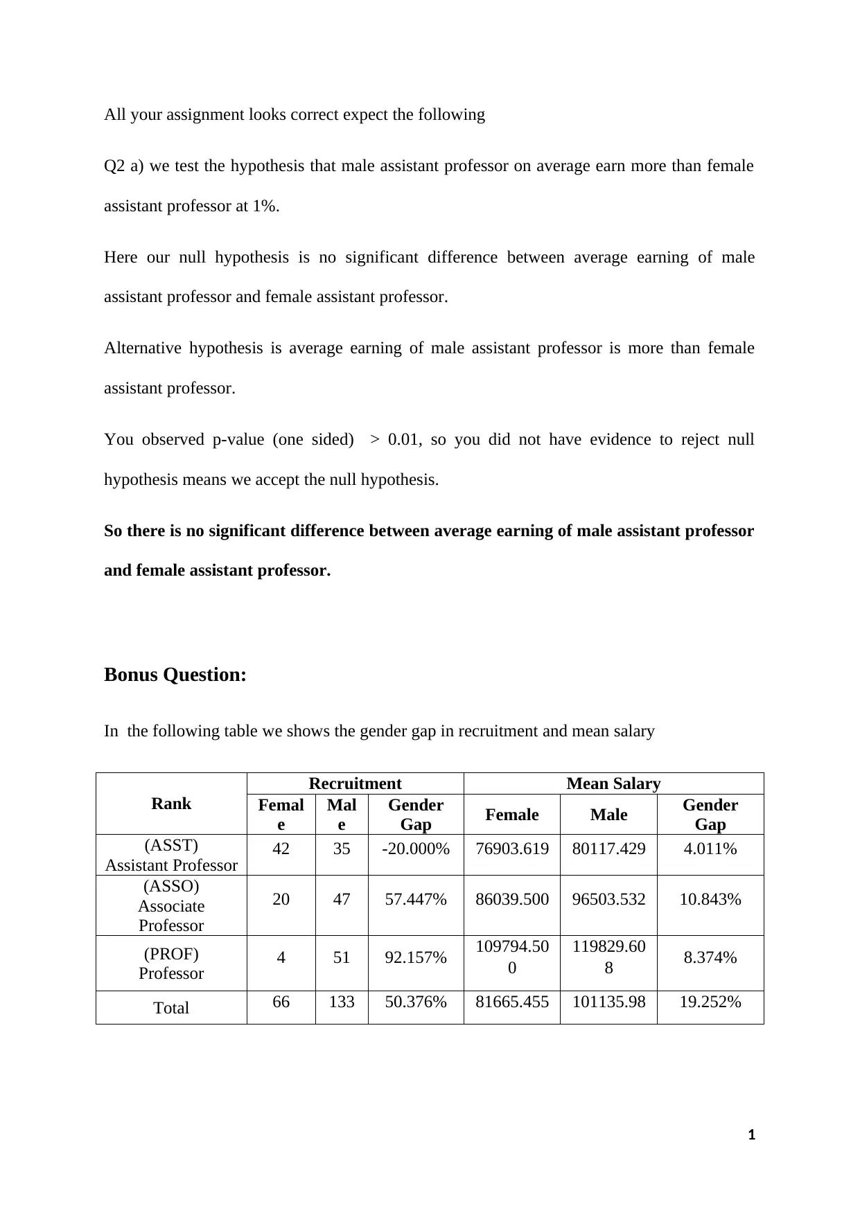
Q2 a) we test the hypothesis that male assistant professor on average earn more than female
assistant professor at 1%.
Here our null hypothesis is no significant difference between average earning of male
assistant professor and female assistant professor.
Alternative hypothesis is average earning of male assistant professor is more than female
assistant professor.
You observed p-value (one sided) > 0.01, so you did not have evidence to reject null
hypothesis means we accept the null hypothesis.
So there is no significant difference between average earning of male assistant professor
and female assistant professor.
Bonus Question:
In the following table we shows the gender gap in recruitment and mean salary
Rank
Recruitment Mean Salary
Femal
e
Mal
e
Gender
Gap Female Male Gender
Gap
(ASST)
Assistant Professor 42 35 -20.000% 76903.619 80117.429 4.011%
(ASSO)
Associate
Professor
20 47 57.447% 86039.500 96503.532 10.843%
(PROF)
Professor 4 51 92.157% 109794.50
0
119829.60
8 8.374%
Total 66 133 50.376% 81665.455 101135.98 19.252%
1

We observed that total gender gap in recruitment is 50.376% whereas rank wise is -
20%, 57.447% and 92.157% for assistant professor, associate professor and professor
respectively. We also observed total gender gap in mean salary is 19.252% whereas gender
gap rank wise is 4.011%, 10.843% and 8.374% for assistant professor, associate professor
and professor respectively.
Yes we can observe the association with Simpson’s paradox as we can see that total gender
gap in mean salary is more than rank wise. It is mainly due to the number of female
academics rank wise.
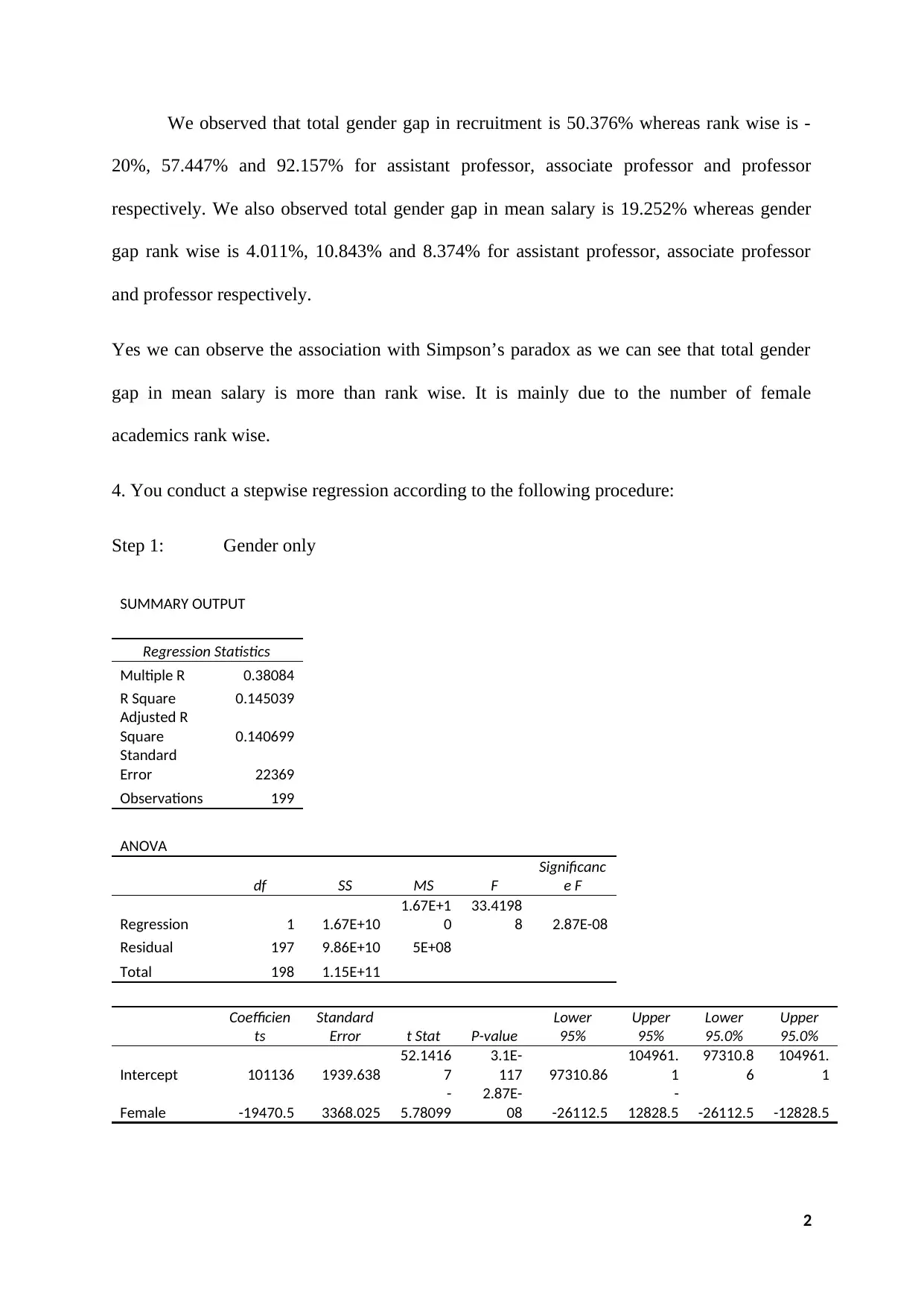
4. You conduct a stepwise regression according to the following procedure:
Step 1: Gender only
SUMMARY OUTPUT
Regression Statistics
Multiple R 0.38084
R Square 0.145039
Adjusted R
Square 0.140699
Standard
Error 22369
Observations 199
ANOVA
df SS MS F
Significanc
e F
Regression 1 1.67E+10
1.67E+1
0
33.4198
8 2.87E-08
Residual 197 9.86E+10 5E+08
Total 198 1.15E+11
Coefficien
ts
Standard
Error t Stat P-value
Lower
95%
Upper
95%
Lower
95.0%
Upper
95.0%
Intercept 101136 1939.638
52.1416
7
3.1E-
117 97310.86
104961.
1
97310.8
6
104961.
1
Female -19470.5 3368.025
-
5.78099
2.87E-
08 -26112.5
-
12828.5 -26112.5 -12828.5
2

Regression Equation:
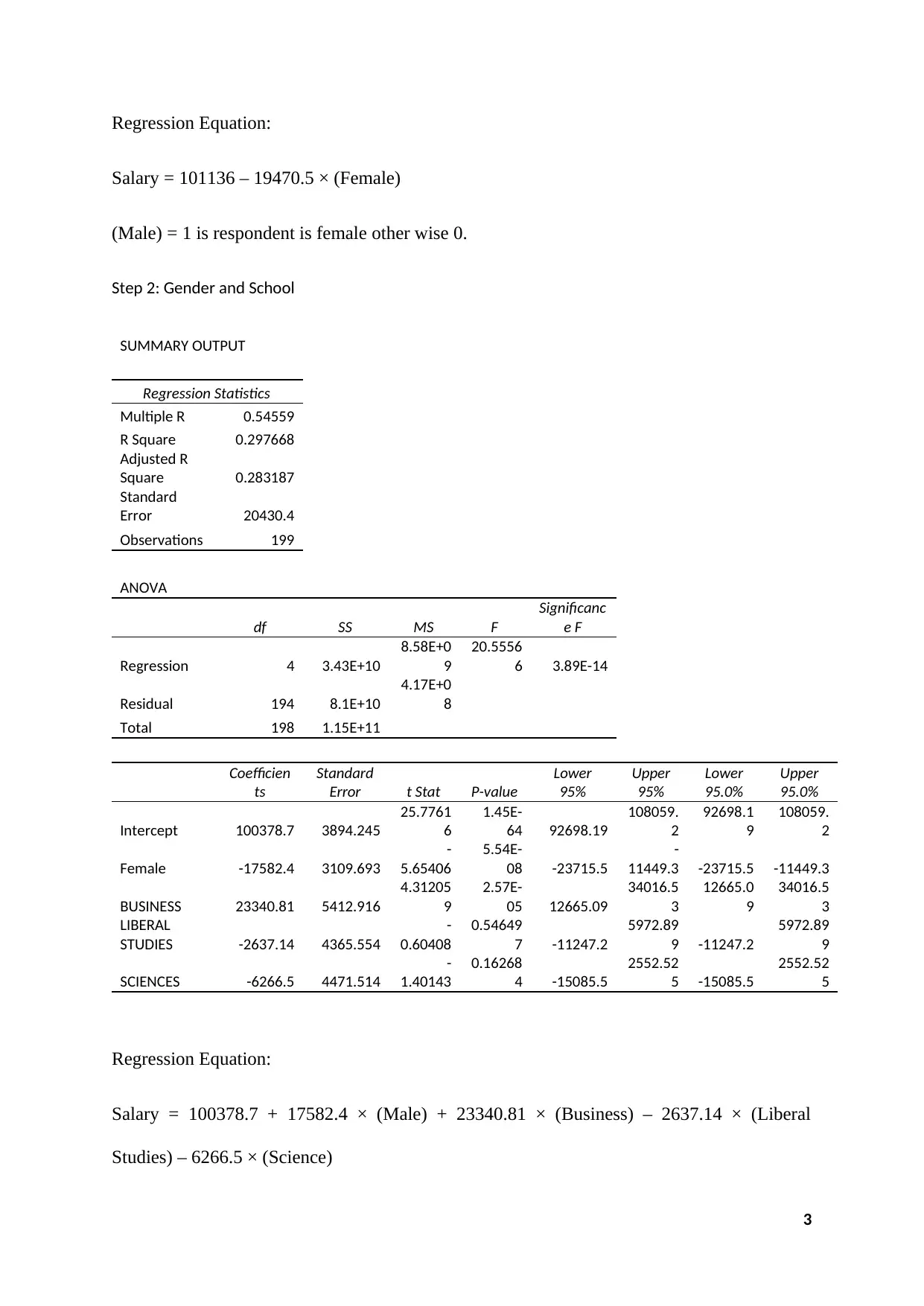
Salary = 101136 – 19470.5 × (Female)
(Male) = 1 is respondent is female other wise 0.
Step 2: Gender and School
SUMMARY OUTPUT
Regression Statistics
Multiple R 0.54559
R Square 0.297668
Adjusted R
Square 0.283187
Standard
Error 20430.4
Observations 199
ANOVA
df SS MS F
Significanc
e F
Regression 4 3.43E+10
8.58E+0
9
20.5556
6 3.89E-14
Residual 194 8.1E+10
4.17E+0
8
Total 198 1.15E+11
Coefficien
ts
Standard
Error t Stat P-value
Lower
95%
Upper
95%
Lower
95.0%
Upper
95.0%
Intercept 100378.7 3894.245
25.7761
6
1.45E-
64 92698.19
108059.
2
92698.1
9
108059.
2
Female -17582.4 3109.693
-
5.65406
5.54E-
08 -23715.5
-
11449.3 -23715.5 -11449.3
BUSINESS 23340.81 5412.916
4.31205
9
2.57E-
05 12665.09
34016.5
3
12665.0
9
34016.5
3
LIBERAL
STUDIES -2637.14 4365.554
-
0.60408
0.54649
7 -11247.2
5972.89
9 -11247.2
5972.89
9
SCIENCES -6266.5 4471.514
-
1.40143
0.16268
4 -15085.5
2552.52
5 -15085.5
2552.52
5
Regression Equation:
Salary = 100378.7 + 17582.4 × (Male) + 23340.81 × (Business) – 2637.14 × (Liberal
Studies) – 6266.5 × (Science)
3

(Female) = 1 is respondent is female other wise 0.
(Business) = 1 if respondent from business school otherwise 0
(Liberal Studies) = 1 if respondent from Liberal Studies school otherwise 0
(Science) = 1 if respondent from Science school otherwise 0
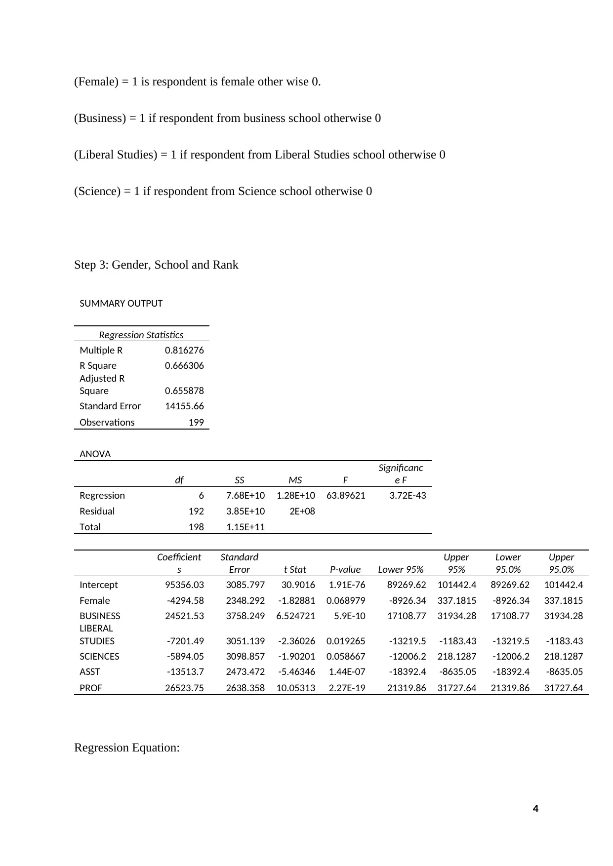
Step 3: Gender, School and Rank
SUMMARY OUTPUT
Regression Statistics
Multiple R 0.816276
R Square 0.666306
Adjusted R
Square 0.655878
Standard Error 14155.66
Observations 199
ANOVA
df SS MS F
Significanc
e F
Regression 6 7.68E+10 1.28E+10 63.89621 3.72E-43
Residual 192 3.85E+10 2E+08
Total 198 1.15E+11
Coefficient
s
Standard
Error t Stat P-value Lower 95%
Upper
95%
Lower
95.0%
Upper
95.0%
Intercept 95356.03 3085.797 30.9016 1.91E-76 89269.62 101442.4 89269.62 101442.4
Female -4294.58 2348.292 -1.82881 0.068979 -8926.34 337.1815 -8926.34 337.1815
BUSINESS 24521.53 3758.249 6.524721 5.9E-10 17108.77 31934.28 17108.77 31934.28
LIBERAL
STUDIES -7201.49 3051.139 -2.36026 0.019265 -13219.5 -1183.43 -13219.5 -1183.43
SCIENCES -5894.05 3098.857 -1.90201 0.058667 -12006.2 218.1287 -12006.2 218.1287
ASST -13513.7 2473.472 -5.46346 1.44E-07 -18392.4 -8635.05 -18392.4 -8635.05
PROF 26523.75 2638.358 10.05313 2.27E-19 21319.86 31727.64 21319.86 31727.64
Regression Equation:
4

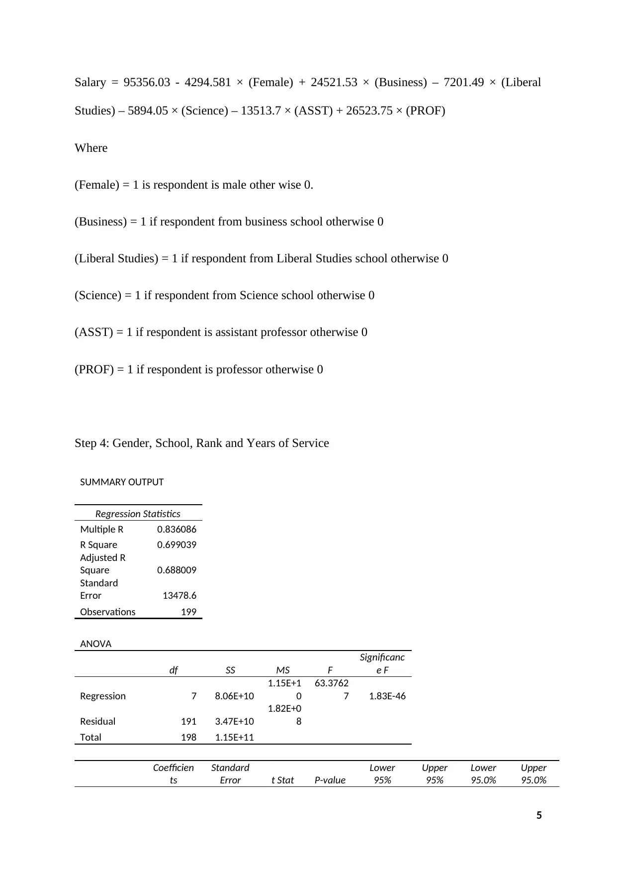
Salary = 95356.03 - 4294.581 × (Female) + 24521.53 × (Business) – 7201.49 × (Liberal
Studies) – 5894.05 × (Science) – 13513.7 × (ASST) + 26523.75 × (PROF)
Where
(Female) = 1 is respondent is male other wise 0.
(Business) = 1 if respondent from business school otherwise 0
(Liberal Studies) = 1 if respondent from Liberal Studies school otherwise 0
(Science) = 1 if respondent from Science school otherwise 0
(ASST) = 1 if respondent is assistant professor otherwise 0
(PROF) = 1 if respondent is professor otherwise 0
Step 4: Gender, School, Rank and Years of Service
SUMMARY OUTPUT
Regression Statistics
Multiple R 0.836086
R Square 0.699039
Adjusted R
Square 0.688009
Standard
Error 13478.6
Observations 199
ANOVA
df SS MS F
Significanc
e F
Regression 7 8.06E+10
1.15E+1
0
63.3762
7 1.83E-46
Residual 191 3.47E+10
1.82E+0
8
Total 198 1.15E+11
Coefficien
ts
Standard
Error t Stat P-value
Lower
95%
Upper
95%
Lower
95.0%
Upper
95.0%
5

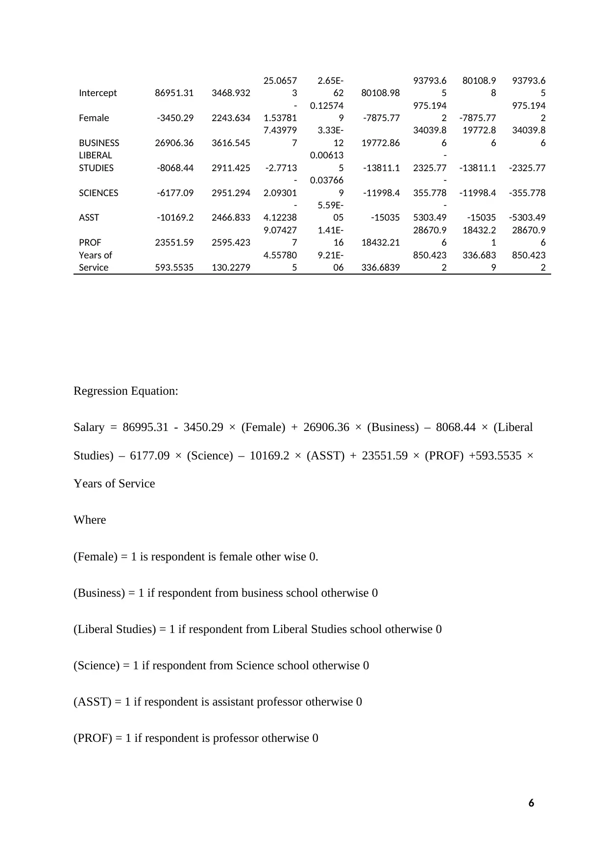
Intercept 86951.31 3468.932
25.0657
3
2.65E-
62 80108.98
93793.6
5
80108.9
8
93793.6
5
Female -3450.29 2243.634
-
1.53781
0.12574
9 -7875.77
975.194
2 -7875.77
975.194
2
BUSINESS 26906.36 3616.545
7.43979
7
3.33E-
12 19772.86
34039.8
6
19772.8
6
34039.8
6
LIBERAL
STUDIES -8068.44 2911.425 -2.7713
0.00613
5 -13811.1
-
2325.77 -13811.1 -2325.77
SCIENCES -6177.09 2951.294
-
2.09301
0.03766
9 -11998.4
-
355.778 -11998.4 -355.778
ASST -10169.2 2466.833
-
4.12238
5.59E-
05 -15035
-
5303.49 -15035 -5303.49
PROF 23551.59 2595.423
9.07427
7
1.41E-
16 18432.21
28670.9
6
18432.2
1
28670.9
6
Years of
Service 593.5535 130.2279
4.55780
5
9.21E-
06 336.6839
850.423
2
336.683
9
850.423
2
Regression Equation:
Salary = 86995.31 - 3450.29 × (Female) + 26906.36 × (Business) – 8068.44 × (Liberal
Studies) – 6177.09 × (Science) – 10169.2 × (ASST) + 23551.59 × (PROF) +593.5535 ×
Years of Service
Where
(Female) = 1 is respondent is female other wise 0.
(Business) = 1 if respondent from business school otherwise 0
(Liberal Studies) = 1 if respondent from Liberal Studies school otherwise 0
(Science) = 1 if respondent from Science school otherwise 0
(ASST) = 1 if respondent is assistant professor otherwise 0
(PROF) = 1 if respondent is professor otherwise 0
6

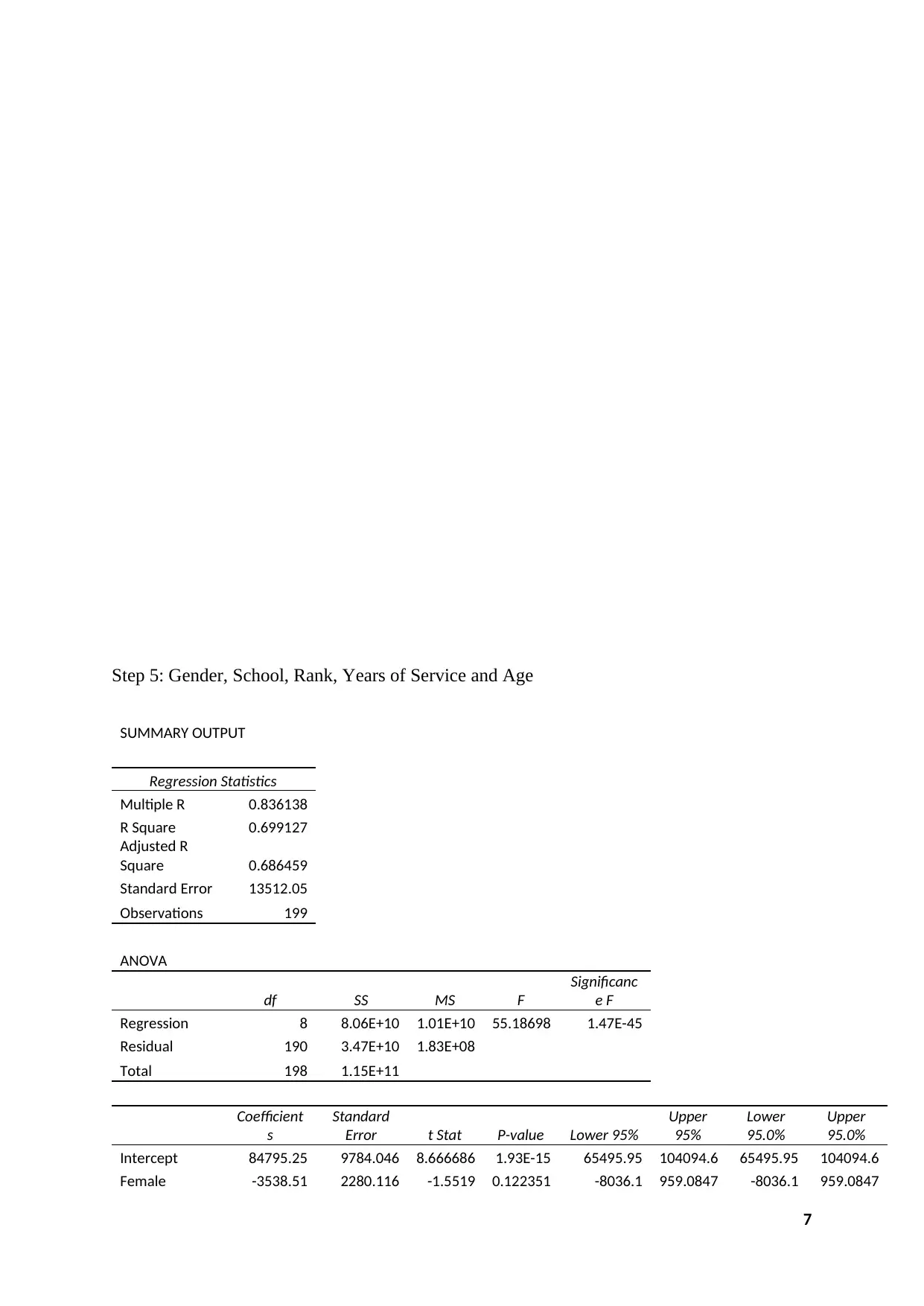
Step 5: Gender, School, Rank, Years of Service and Age
SUMMARY OUTPUT
Regression Statistics
Multiple R 0.836138
R Square 0.699127
Adjusted R
Square 0.686459
Standard Error 13512.05
Observations 199
ANOVA
df SS MS F
Significanc
e F
Regression 8 8.06E+10 1.01E+10 55.18698 1.47E-45
Residual 190 3.47E+10 1.83E+08
Total 198 1.15E+11
Coefficient
s
Standard
Error t Stat P-value Lower 95%
Upper
95%
Lower
95.0%
Upper
95.0%
Intercept 84795.25 9784.046 8.666686 1.93E-15 65495.95 104094.6 65495.95 104094.6
Female -3538.51 2280.116 -1.5519 0.122351 -8036.1 959.0847 -8036.1 959.0847
7

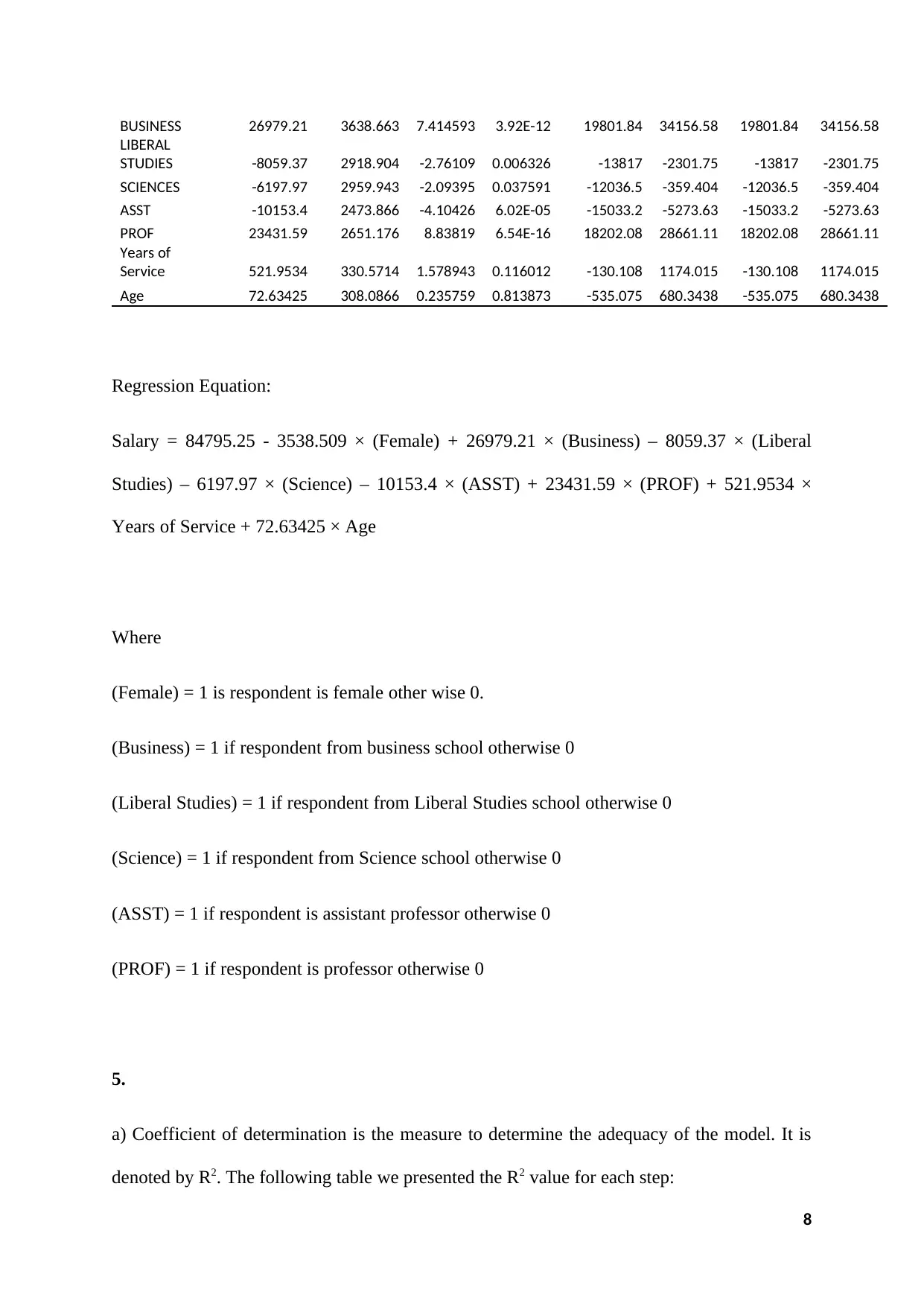
BUSINESS 26979.21 3638.663 7.414593 3.92E-12 19801.84 34156.58 19801.84 34156.58
LIBERAL
STUDIES -8059.37 2918.904 -2.76109 0.006326 -13817 -2301.75 -13817 -2301.75
SCIENCES -6197.97 2959.943 -2.09395 0.037591 -12036.5 -359.404 -12036.5 -359.404
ASST -10153.4 2473.866 -4.10426 6.02E-05 -15033.2 -5273.63 -15033.2 -5273.63
PROF 23431.59 2651.176 8.83819 6.54E-16 18202.08 28661.11 18202.08 28661.11
Years of
Service 521.9534 330.5714 1.578943 0.116012 -130.108 1174.015 -130.108 1174.015
Age 72.63425 308.0866 0.235759 0.813873 -535.075 680.3438 -535.075 680.3438
Regression Equation:
Salary = 84795.25 - 3538.509 × (Female) + 26979.21 × (Business) – 8059.37 × (Liberal
Studies) – 6197.97 × (Science) – 10153.4 × (ASST) + 23431.59 × (PROF) + 521.9534 ×
Years of Service + 72.63425 × Age
Where
(Female) = 1 is respondent is female other wise 0.
(Business) = 1 if respondent from business school otherwise 0
(Liberal Studies) = 1 if respondent from Liberal Studies school otherwise 0
(Science) = 1 if respondent from Science school otherwise 0
(ASST) = 1 if respondent is assistant professor otherwise 0
(PROF) = 1 if respondent is professor otherwise 0
5.
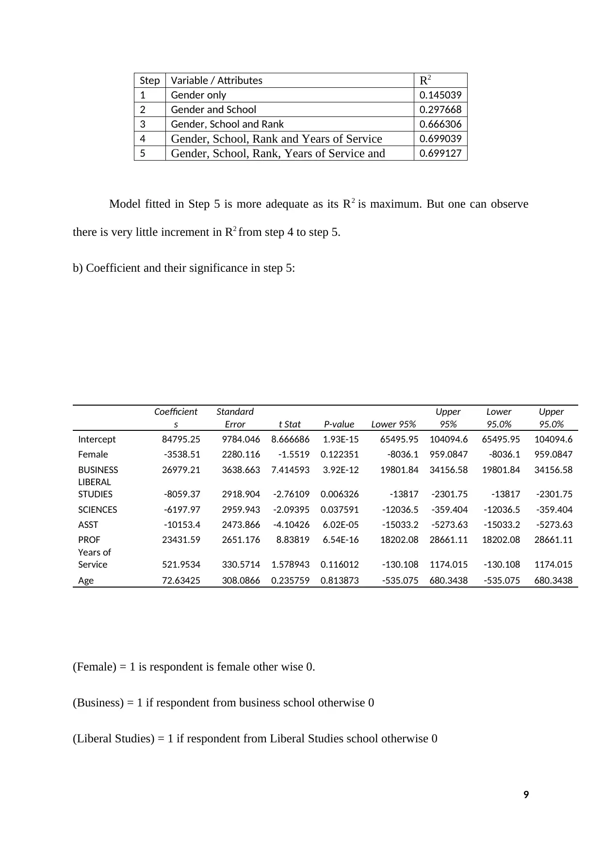
a) Coefficient of determination is the measure to determine the adequacy of the model. It is
denoted by R2. The following table we presented the R2 value for each step:
8

Step Variable / Attributes R2
1 Gender only 0.145039
2 Gender and School 0.297668
3 Gender, School and Rank 0.666306
4 Gender, School, Rank and Years of Service 0.699039
5 Gender, School, Rank, Years of Service and
Age
0.699127
Model fitted in Step 5 is more adequate as its R2 is maximum. But one can observe
there is very little increment in R2 from step 4 to step 5.
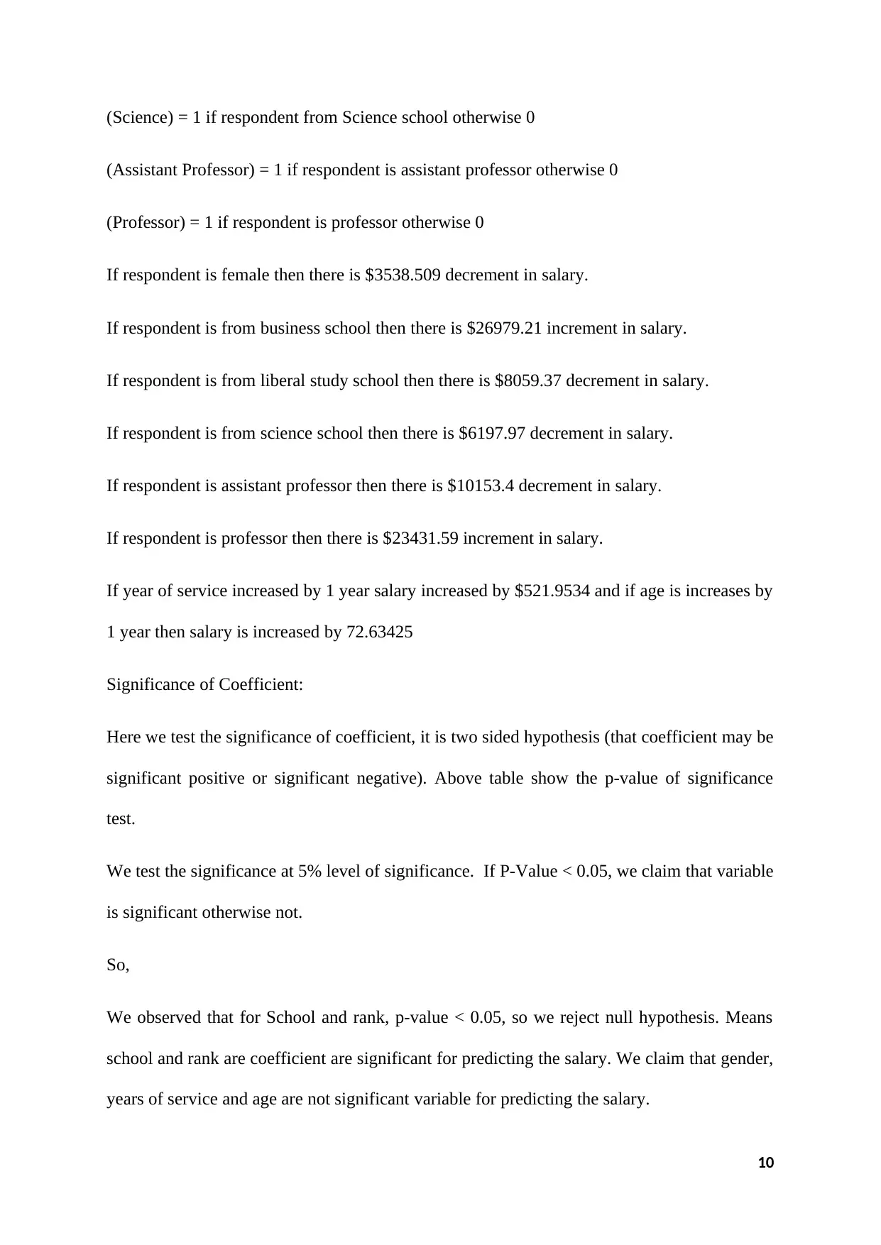
b) Coefficient and their significance in step 5:
Coefficient
s
Standard
Error t Stat P-value Lower 95%
Upper
95%
Lower
95.0%
Upper
95.0%
Intercept 84795.25 9784.046 8.666686 1.93E-15 65495.95 104094.6 65495.95 104094.6
Female -3538.51 2280.116 -1.5519 0.122351 -8036.1 959.0847 -8036.1 959.0847
BUSINESS 26979.21 3638.663 7.414593 3.92E-12 19801.84 34156.58 19801.84 34156.58
LIBERAL
STUDIES -8059.37 2918.904 -2.76109 0.006326 -13817 -2301.75 -13817 -2301.75
SCIENCES -6197.97 2959.943 -2.09395 0.037591 -12036.5 -359.404 -12036.5 -359.404
ASST -10153.4 2473.866 -4.10426 6.02E-05 -15033.2 -5273.63 -15033.2 -5273.63
PROF 23431.59 2651.176 8.83819 6.54E-16 18202.08 28661.11 18202.08 28661.11
Years of
Service 521.9534 330.5714 1.578943 0.116012 -130.108 1174.015 -130.108 1174.015
Age 72.63425 308.0866 0.235759 0.813873 -535.075 680.3438 -535.075 680.3438
(Female) = 1 is respondent is female other wise 0.
(Business) = 1 if respondent from business school otherwise 0
(Liberal Studies) = 1 if respondent from Liberal Studies school otherwise 0
9

(Science) = 1 if respondent from Science school otherwise 0
(Assistant Professor) = 1 if respondent is assistant professor otherwise 0
(Professor) = 1 if respondent is professor otherwise 0
If respondent is female then there is $3538.509 decrement in salary.
If respondent is from business school then there is $26979.21 increment in salary.
If respondent is from liberal study school then there is $8059.37 decrement in salary.
If respondent is from science school then there is $6197.97 decrement in salary.
If respondent is assistant professor then there is $10153.4 decrement in salary.
If respondent is professor then there is $23431.59 increment in salary.
If year of service increased by 1 year salary increased by $521.9534 and if age is increases by
1 year then salary is increased by 72.63425
Significance of Coefficient:
Here we test the significance of coefficient, it is two sided hypothesis (that coefficient may be
significant positive or significant negative). Above table show the p-value of significance
test.
We test the significance at 5% level of significance. If P-Value < 0.05, we claim that variable
is significant otherwise not.
So,
We observed that for School and rank, p-value < 0.05, so we reject null hypothesis. Means
school and rank are coefficient are significant for predicting the salary. We claim that gender,
years of service and age are not significant variable for predicting the salary.
10

6.
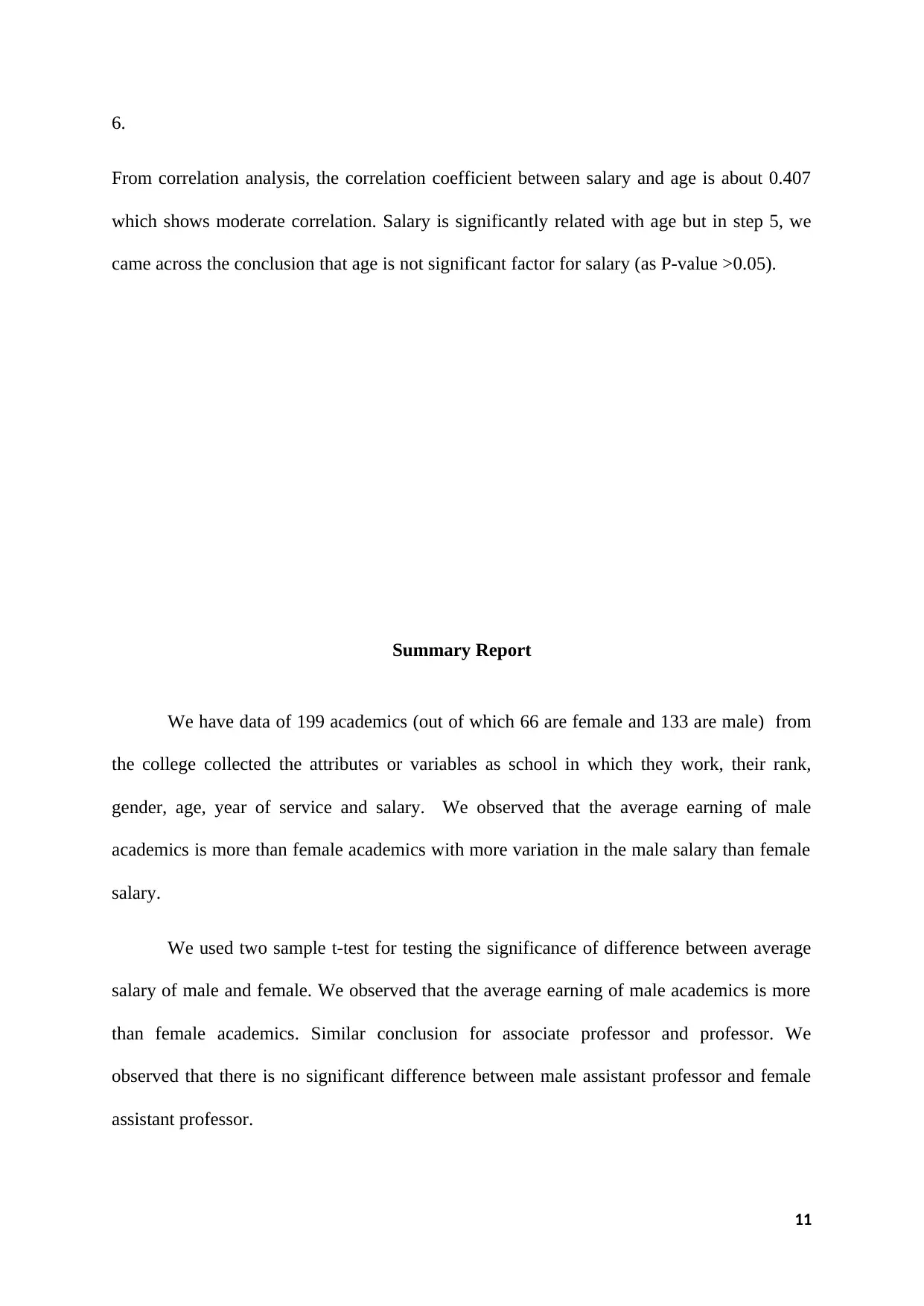
From correlation analysis, the correlation coefficient between salary and age is about 0.407
which shows moderate correlation. Salary is significantly related with age but in step 5, we
came across the conclusion that age is not significant factor for salary (as P-value >0.05).
Summary Report
We have data of 199 academics (out of which 66 are female and 133 are male) from
the college collected the attributes or variables as school in which they work, their rank,
gender, age, year of service and salary. We observed that the average earning of male
academics is more than female academics with more variation in the male salary than female
salary.
We used two sample t-test for testing the significance of difference between average
salary of male and female. We observed that the average earning of male academics is more
than female academics. Similar conclusion for associate professor and professor. We
observed that there is no significant difference between male assistant professor and female
assistant professor.
11

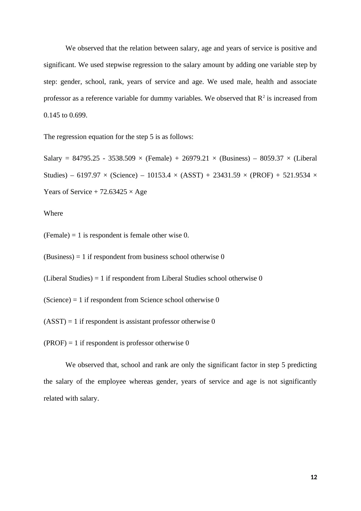
We observed that the relation between salary, age and years of service is positive and
significant. We used stepwise regression to the salary amount by adding one variable step by
step: gender, school, rank, years of service and age. We used male, health and associate
professor as a reference variable for dummy variables. We observed that R2 is increased from
0.145 to 0.699.
The regression equation for the step 5 is as follows:
Salary = 84795.25 - 3538.509 × (Female) + 26979.21 × (Business) – 8059.37 × (Liberal
Studies) – 6197.97 × (Science) – 10153.4 × (ASST) + 23431.59 × (PROF) + 521.9534 ×
Years of Service + 72.63425 × Age
Where
(Female) = 1 is respondent is female other wise 0.
(Business) = 1 if respondent from business school otherwise 0
(Liberal Studies) = 1 if respondent from Liberal Studies school otherwise 0
(Science) = 1 if respondent from Science school otherwise 0
(ASST) = 1 if respondent is assistant professor otherwise 0
(PROF) = 1 if respondent is professor otherwise 0
We observed that, school and rank are only the significant factor in step 5 predicting
the salary of the employee whereas gender, years of service and age is not significantly
related with salary.
12

References:
Bickel, P. J., & Doksum, K. A. (2015). Mathematical statistics: basic ideas and selected
topics, volume I (Vol. 117). CRC Press.
Box, G. E., Hunter, J. S., & Hunter, W. G. (2005). Statistics for experimenters: design,
innovation, and discovery (Vol. 2). New York: Wiley-Interscience.
Chatterjee, S., & Hadi, A. S. (2015). Regression analysis by example. John Wiley & Sons.
Devore, J. L., & Berk, K. N. (2007). Modern mathematical statistics with applications.
Cengage Learning.
Draper, N. R., & Smith, H. (2014). Applied regression analysis (Vol. 326). John Wiley &
Sons.
13

Larsen, R. J., & Marx, M. L. (2017). An introduction to mathematical statistics and its
applications (Vol. 5). Pearson.
Levine, D. M., Berenson, M. L., Stephan, D., & Lysell, D. (1999). Statistics for managers
using Microsoft Excel (Vol. 660). Upper Saddle River, NJ: Prentice Hall.
Moyé, L. A., Chan, W., & Kapadia, A. S. (2017). Mathematical statistics with applications.
CRC Press.
Ramachandran, K. M., & Tsokos, C. P. (2014). Mathematical statistics with applications in
R. Elsevier.
Ryan, T. P. (2008). Modern regression methods (Vol. 655). John Wiley & Sons.
Triola, M. F. (2013). Elementary statistics using Excel. Pearson.
14