SEO for Desklib: Title, Meta Title, Meta Description, Slug, Summary, Subject, Course Code, Course Name, College/University

Desklib is an online library for study material that provides access to solved assignments, essays, dissertations and more. The meta title and description highlight the key features of Desklib and its offerings. The slug is simple and relevant to the content for SEO purposes. The subject, course code, course name and college/university are not mentioned in the given content.

Running Head: STATISTICS
Statistics
Name of the Student
Name of the University
Author Note

1STATISTICS
Table of Contents
ANSWER 1.....................................................................................................................................3
Part a............................................................................................................................................3
Part b............................................................................................................................................3
Part c............................................................................................................................................4
ANSWER 2.....................................................................................................................................4
Part a............................................................................................................................................4
Part b............................................................................................................................................4
Part c............................................................................................................................................5
Part d............................................................................................................................................6
ANSWER 3.....................................................................................................................................7
Part a............................................................................................................................................7
Part b............................................................................................................................................8
ANSWER 4.....................................................................................................................................8
Part a............................................................................................................................................8
Part b............................................................................................................................................8
Part c............................................................................................................................................8
Part d............................................................................................................................................8
ANSWER 5.....................................................................................................................................9

2STATISTICS
ANSWER 6...................................................................................................................................10
ANSWER 7...................................................................................................................................10
Part a..........................................................................................................................................11
Part b..........................................................................................................................................11
Part c..........................................................................................................................................11
ANSWER 8...................................................................................................................................12

3STATISTICS
ANSWER 1
Part a
Class Interval Frequency Relative
Freqency
Cumulative
Relative
Frequency
Class
Midpoint
0 - 65 7 0.117 0.117 32.5
65 - 130 11 0.183 0.300 97.5
130 - 195 15 0.250 0.550 162.5
195 - 260 11 0.183 0.733 227.5
260 - 325 8 0.133 0.867 292.5
325 - 390 0 0.000 0.867 357.5
390 - 455 5 0.083 0.950 422.5
455 - 520 0 0.000 0.950 487.5
520 - 585 2 0.033 0.983 552.5
585 - 650 1 0.017 1.000 617.5
Total 60
Part b
0 - 65
65 - 130
130 - 195
195 - 260
260 - 325
325 - 390
390 - 455
455 - 520
520 - 585
585 - 6500
2
4
6
8
10
12
14
16
Distribution of Prices
Price Range
Frequency
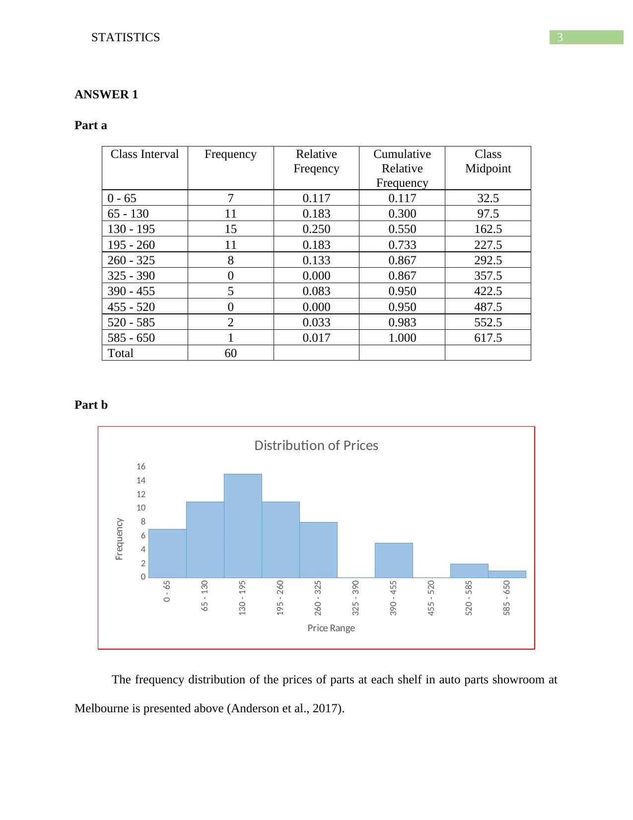
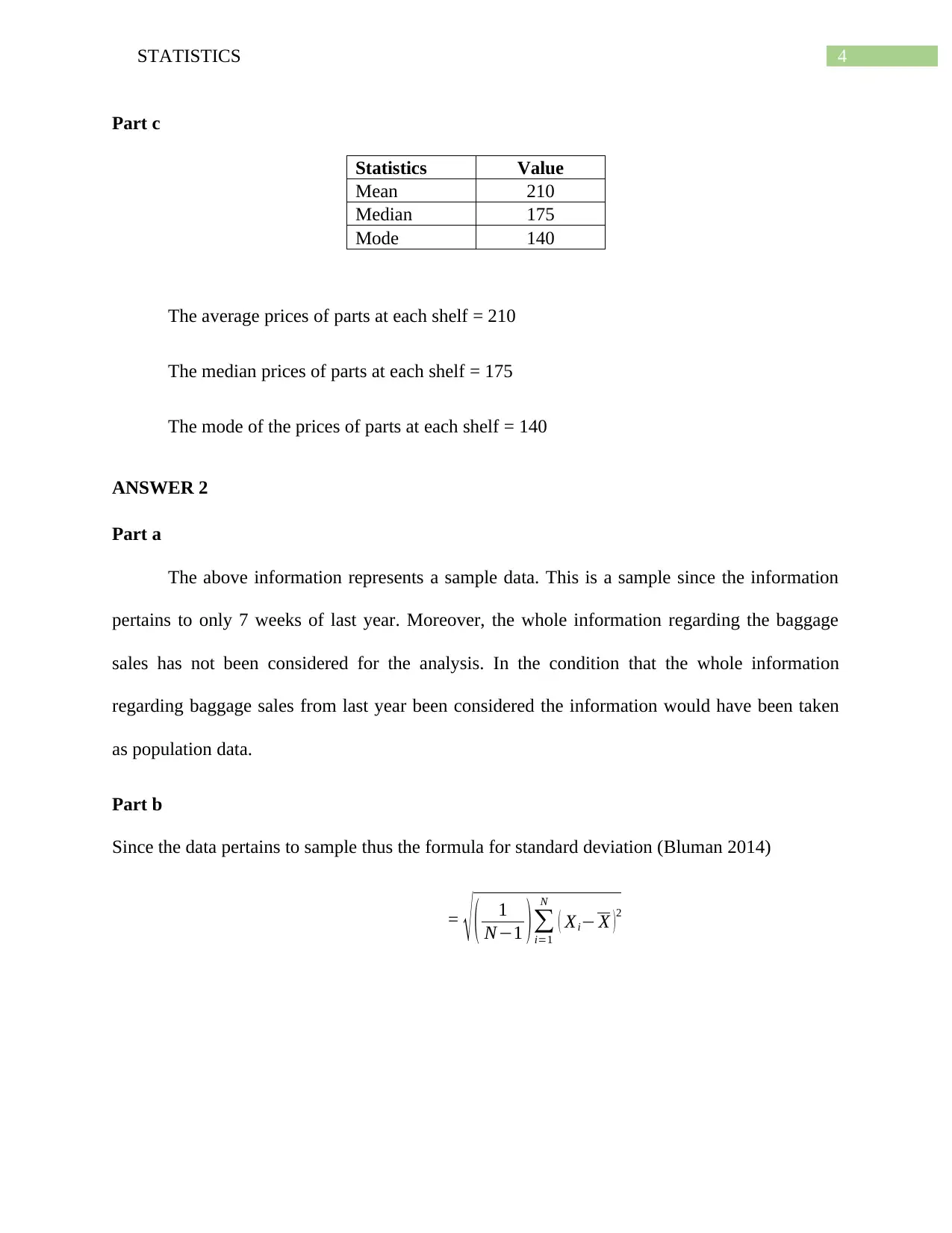
The frequency distribution of the prices of parts at each shelf in auto parts showroom at
Melbourne is presented above (Anderson et al., 2017).

4STATISTICS
Part c
Statistics Value
Mean 210
Median 175
Mode 140
The average prices of parts at each shelf = 210
The median prices of parts at each shelf = 175
The mode of the prices of parts at each shelf = 140
ANSWER 2
Part a
The above information represents a sample data. This is a sample since the information
pertains to only 7 weeks of last year. Moreover, the whole information regarding the baggage
sales has not been considered for the analysis. In the condition that the whole information
regarding baggage sales from last year been considered the information would have been taken
as population data.
Part b
Since the data pertains to sample thus the formula for standard deviation (Bluman 2014)
= √ ( 1
N−1 )∑
i=1
N
( Xi− X )2

5STATISTICS
Statistics Number of flights at the airport (Xi −X ) ( X i−X )2
30 1.286 1.65
25 -3.714 13.80
20 -8.714 75.94
27 -1.714 2.94
34 5.286 27.94
33 4.286 18.37
32 3.286 10.80
Sum 201 172.286 151.43
Average 28.714
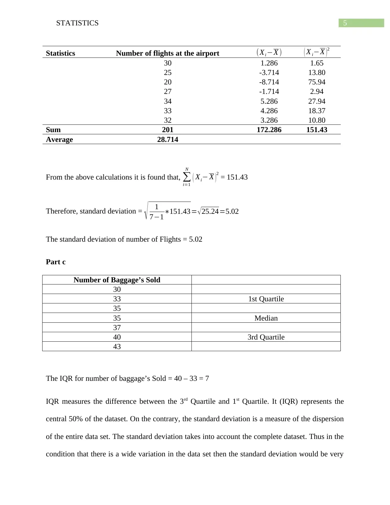
From the above calculations it is found that, ∑
i=1
N
( Xi− X )
2 = 151.43
Therefore, standard deviation = √ 1
7−1∗151.43= √ 25.24=5.02
The standard deviation of number of Flights = 5.02
Part c
Number of Baggage’s Sold
30
33 1st Quartile
35
35 Median
37
40 3rd Quartile
43
The IQR for number of baggage’s Sold = 40 – 33 = 7
IQR measures the difference between the 3rd Quartile and 1st Quartile. It (IQR) represents the
central 50% of the dataset. On the contrary, the standard deviation is a measure of the dispersion
of the entire data set. The standard deviation takes into account the complete dataset. Thus in the
condition that there is a wide variation in the data set then the standard deviation would be very

6STATISTICS
high. However, if there is very less deviation in the central 50% then the IQR would be less. In
addition, if outliers are present then also standard deviation may be high.
Let’s assume that in the first week the number of baggage’s sold is 0 and in any week 100
baggage’s were sold. Then, the standard deviation would increase drastically. But the IQR would
remain the same.
Part d
Number of
flights at the
airport (x)
Number of
baggage’s sold (y)
xy x2 y2
30 30 900 900 900
25 33 825 625 1089
20 35 700 400 1225
27 35 945 729 1225
34 37 1258 1156 1369
33 40 1320 1089 1600
32 43 1376 1024 1849
201 253 7324 5923 9257
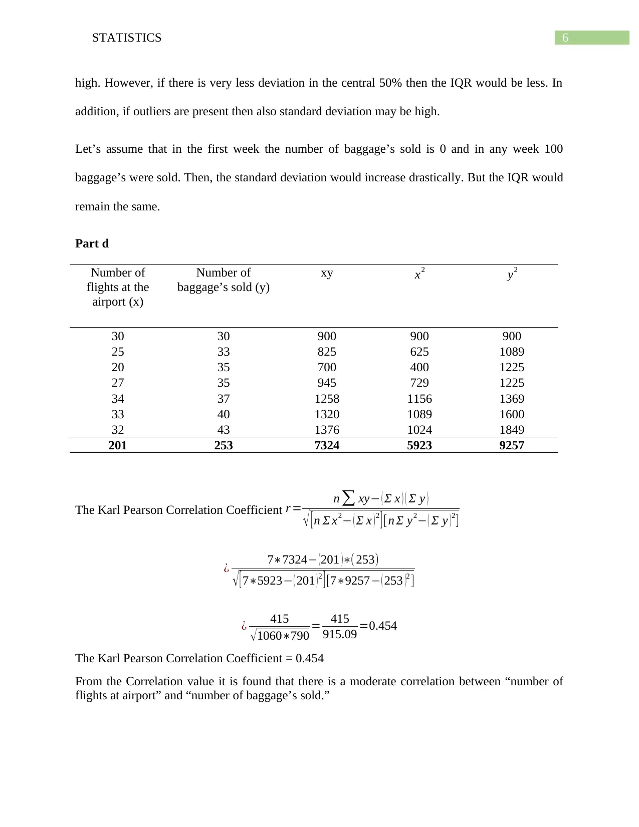
The Karl Pearson Correlation Coefficient r = n ∑ xy− ( Σ x ) ( Σ y )
√ [ n Σ x2− ( Σ x )2 ] [n Σ y2− ( Σ y )2]
¿ 7∗7324− (201 )∗( 253)
√ [ 7∗5923− ( 201 )2 ] [7∗9257− ( 253 )2 ]
¿ 415
√1060∗790 = 415
915.09 =0.454
The Karl Pearson Correlation Coefficient = 0.454
From the Correlation value it is found that there is a moderate correlation between “number of
flights at airport” and “number of baggage’s sold.”

7STATISTICS

8STATISTICS
ANSWER 3
Part a
For the baggage stores the number of flights is the independent variable and the number of
baggage sold is the dependent variable.
Number of
flights at the
airport (x)
Number of
baggage’s
sold (y)
( xi−x ) ( yi− y) ( xi−x )∗( yi− y)( xi−x )
2
( yi− y )2
30 30 1.29 -6.14 -7.90 1.65 37.73
25 33 -3.71 -3.14 11.67 13.80 9.88
20 35 -8.71 -1.14 9.96 75.94 1.31
27 35 -1.71 -1.14 1.96 2.94 1.31
34 37 5.29 0.86 4.53 27.94 0.73
33 40 4.29 3.86 16.53 18.37 14.88
32 43 3.29 6.86 22.53 10.80 47.02
Sum 201 253 59.29 151.43 112.86
Average
28.71 36.14
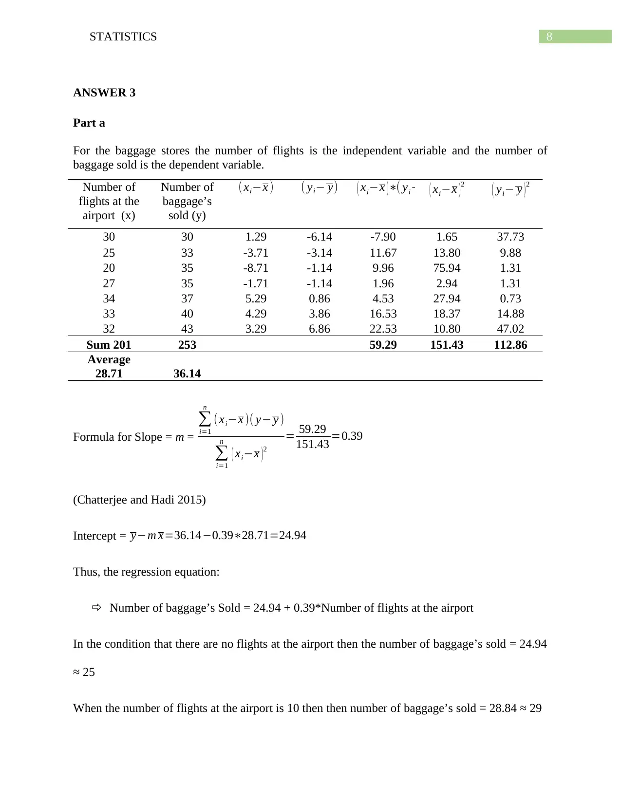
Formula for Slope = m =
∑
i=1
n
(xi−x )( y− y )
∑
i=1
n
( xi−x )2
= 59.29
151.43 =0.39
(Chatterjee and Hadi 2015)
Intercept = y−m x=36.14−0.39∗28.71=24.94
Thus, the regression equation:
 Number of baggage’s Sold = 24.94 + 0.39*Number of flights at the airport
In the condition that there are no flights at the airport then the number of baggage’s sold = 24.94
≈ 25
When the number of flights at the airport is 10 then then number of baggage’s sold = 28.84 ≈ 29

9STATISTICS

10STATISTICS
Part b
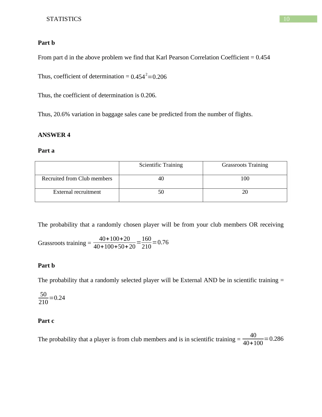
From part d in the above problem we find that Karl Pearson Correlation Coefficient = 0.454
Thus, coefficient of determination = 0.4542=0.206
Thus, the coefficient of determination is 0.206.
Thus, 20.6% variation in baggage sales cane be predicted from the number of flights.
ANSWER 4
Part a
Scientific Training Grassroots Training
Recruited from Club members 40 100
External recruitment 50 20
The probability that a randomly chosen player will be from your club members OR receiving
Grassroots training = 40+100+20
40+100+50+ 20 =160
210 =0.76
Part b
The probability that a randomly selected player will be External AND be in scientific training =
50
210 =0.24
Part c
The probability that a player is from club members and is in scientific training = 40
40+100 =0.286

11STATISTICS
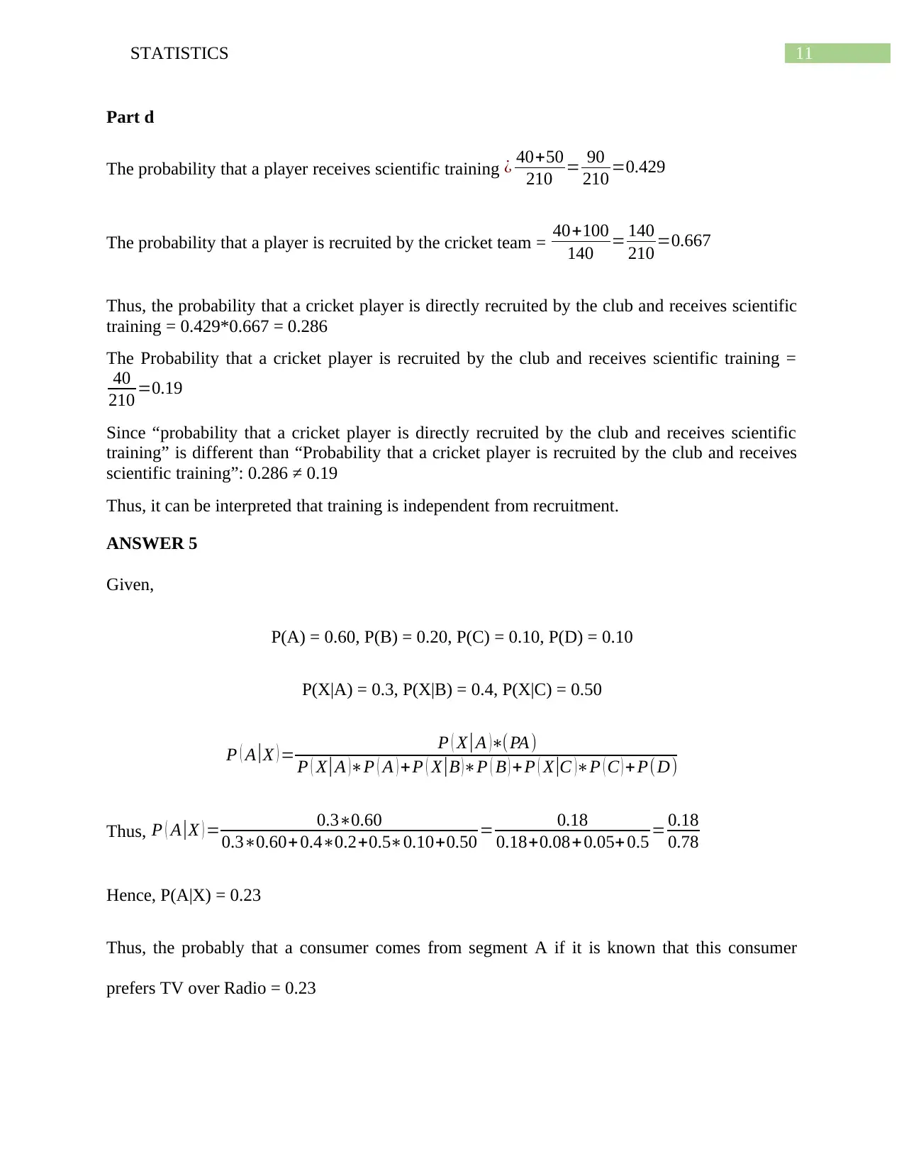
Part d
The probability that a player receives scientific training ¿ 40+50
210 = 90
210 =0.429
The probability that a player is recruited by the cricket team = 40+100
140 = 140
210 =0.667
Thus, the probability that a cricket player is directly recruited by the club and receives scientific
training = 0.429*0.667 = 0.286
The Probability that a cricket player is recruited by the club and receives scientific training =
40
210 =0.19
Since “probability that a cricket player is directly recruited by the club and receives scientific
training” is different than “Probability that a cricket player is recruited by the club and receives
scientific training”: 0.286 ≠ 0.19
Thus, it can be interpreted that training is independent from recruitment.
ANSWER 5
Given,
P(A) = 0.60, P(B) = 0.20, P(C) = 0.10, P(D) = 0.10
P(X|A) = 0.3, P(X|B) = 0.4, P(X|C) = 0.50
P ( A |X ) = P ( X | A )∗(PA)
P ( X | A )∗P ( A ) + P ( X |B )∗P ( B ) + P ( X |C )∗P ( C ) + P(D)
Thus, P ( A |X ) = 0.3∗0.60
0.3∗0.60+0.4∗0.2+0.5∗0.10+0.50 = 0.18
0.18+0.08+0.05+ 0.5 = 0.18
0.78
Hence, P(A|X) = 0.23
Thus, the probably that a consumer comes from segment A if it is known that this consumer
prefers TV over Radio = 0.23

12STATISTICS

13STATISTICS
ANSWER 6
Price (x) Probability P(x) Mean standard
Deviation
1000 0.00004 0.04000 39.94607
100 0.00070 0.07000 6.90591
20 0.00530 0.10600 1.97945
10 0.00711 0.07110 0.61834
4 0.02003 0.08012 0.22153
2 0.09180 0.18360 0.16133
1 0.12350 0.12350 0.01310
0 0.76417 0.00000 0.34747
0.67432 50.19322
7.08472
The mean amount is calculated as Σ xP (x)
The mean amount won per ticket = 0.67432
The mean value represents the average amount that a person can expect to win by purchasing a
ticket of $2.
The standard deviation of the amount is calculated as √ Σ ( x−μ ) 2 P ( x )
The standard deviation of the amount won per ticket = 7.08472
The amount of tickets sold = 2million * 2$ = $4,000,000
The total amount won by the customers = 2million*0.67432 = $1348640
Thus, the expected profit from the festival = $4,000,000 - $1348640 = $2651360
ANSWER 7
The mean speed of the train = 250 km per hour

14STATISTICS
The standard deviation of the speed of the train = 30 km per hour
Part a
The probability that the speed would be less than 200 km per hour
Z= X−μ
σ = 200−250
30 =−50
30 =−1.667
P(Z<-1.667) = 0.048
Thus, the probability that the speed would be less than 200 km per hour = 0.048
Part b
The probability that the speed would be more than 300 km per hour
Z= X−μ
σ = 300−250
30 =50
30 =1.667
P(Z > 1.667) = 1 - 0.952 = 0.048
Thus, the probability that the speed would be less than 300 km per hour = 0.048
Part c
The probability that the speed would lie between 210 and 280 km per hour
P ( 210< X <280 )
z= 210−250
30 =−40
30 =−1.33
z= 280−250
30 =30
30 =1.00
P ( 210<X <280 ) =P ( −1.33< z< 1.00 ) =0.408+ 0.341

15STATISTICS
= 0.749
Thus, the probability that the speed lies between 210 and 280 km per hour = 0.749
ANSWER 8
The average number of shoppers = 448
The standard deviation of the shoppers = 21
Thus, the probability that the number of shoppers would lie between 441 and 446
P ( 441< X <446 )
z= 441−448
21 / √ 49 =−2.333
z= 446−448
21/√ 49 =−0.067
P ( 441< X <446 ) =P (−2.333< z←0.067 )=0.010+0.473
= 0.483
Thus, the probability that a random sample of 49 different one-hour shopping periods the mean
number of shoppers would lie between 441 and 446 = 0.483

16STATISTICS
Reference
Anderson, D.R., Sweeney, D.J., Williams, T.A., Camm, J.D. and Cochran, J.J., 2017. Essentials
of Modern Business Statistics With Microsoft Excel.. Cengage Learning
Bluman, A.G., 2014. Elementary statistics: A step by step approach. New York: McGraw-Hill
Higher Education.
Chatterjee, S. and Hadi, A.S., 2015. Regression analysis by example. John Wiley & Sons.