Descriptive and Inferential Statistics Analysis for Desklib

This analysis provides a descriptive and inferential statistics analysis for Desklib, an online library for study material with solved assignments, essays, dissertation etc. It includes means, frequencies, depression score, outliers, and ANOVA results. The analysis is presented in APA format with figures and tables.

Statistics
Student Name:
Instructor Name:
Course Number:
2 September 2018

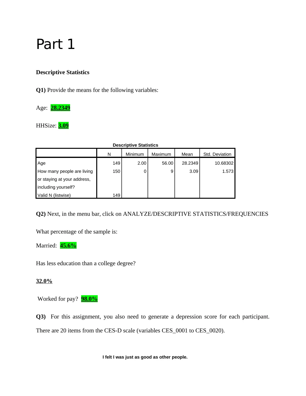
Part 1
Descriptive Statistics
Q1) Provide the means for the following variables:
Age: 28.2349
HHSize: 3.09
Descriptive Statistics
N Minimum Maximum Mean Std. Deviation
Age 149 2.00 56.00 28.2349 10.68302
How many people are living
or staying at your address,
including yourself?
150 0 9 3.09 1.573
Valid N (listwise) 149
Q2) Next, in the menu bar, click on ANALYZE/DESCRIPTIVE STATISTICS/FREQUENCIES
What percentage of the sample is:
Married: 45.6%
Has less education than a college degree?
32.0%
Worked for pay? 98.0%
Q3) For this assignment, you also need to generate a depression score for each participant.
There are 20 items from the CES-D scale (variables CES_0001 to CES_0020).
I felt I was just as good as other people.

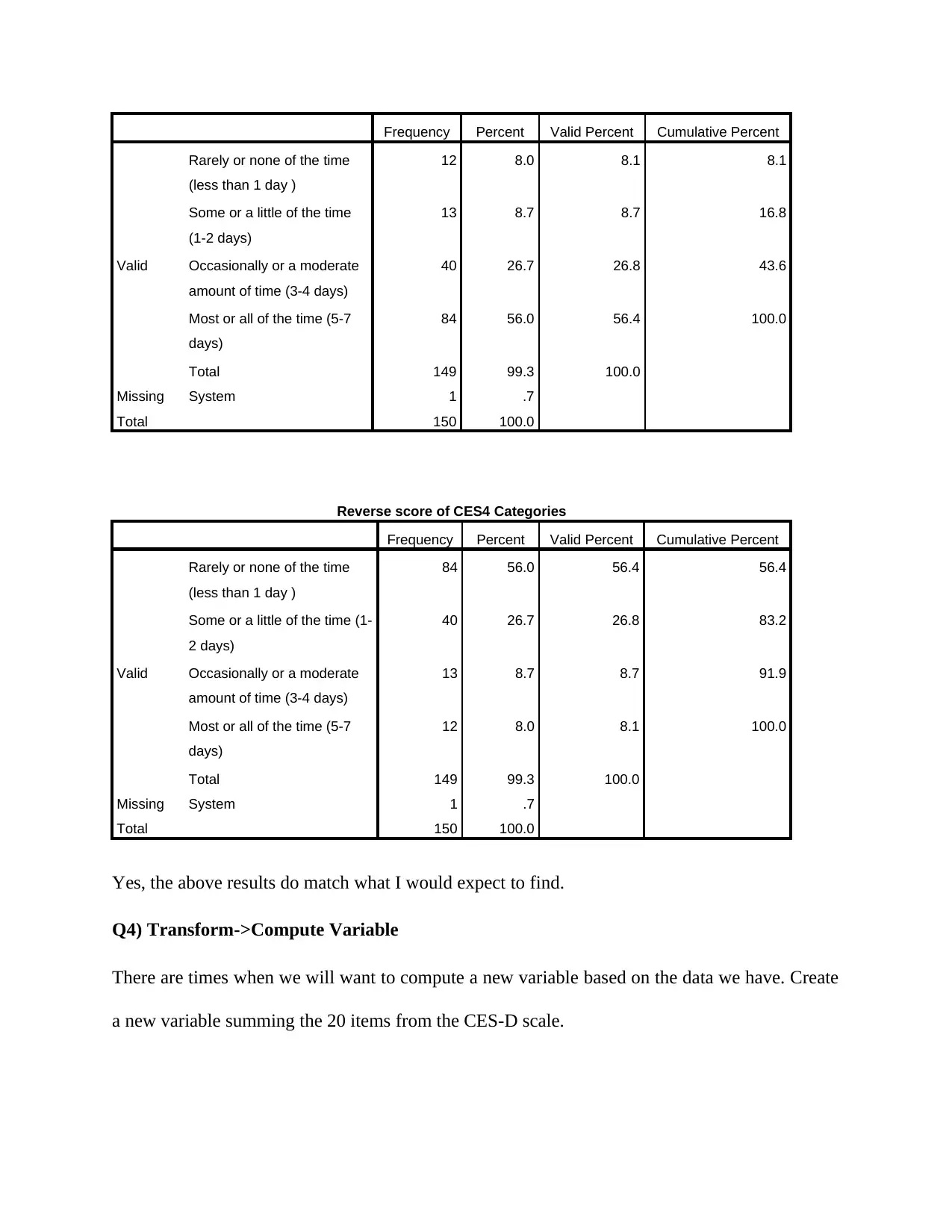
Frequency Percent Valid Percent Cumulative Percent
Valid
Rarely or none of the time
(less than 1 day )
12 8.0 8.1 8.1
Some or a little of the time
(1-2 days)
13 8.7 8.7 16.8
Occasionally or a moderate
amount of time (3-4 days)
40 26.7 26.8 43.6
Most or all of the time (5-7
days)
84 56.0 56.4 100.0
Total 149 99.3 100.0
Missing System 1 .7
Total 150 100.0
Reverse score of CES4 Categories
Frequency Percent Valid Percent Cumulative Percent
Valid
Rarely or none of the time
(less than 1 day )
84 56.0 56.4 56.4
Some or a little of the time (1-
2 days)
40 26.7 26.8 83.2
Occasionally or a moderate
amount of time (3-4 days)
13 8.7 8.7 91.9
Most or all of the time (5-7
days)
12 8.0 8.1 100.0
Total 149 99.3 100.0
Missing System 1 .7
Total 150 100.0
Yes, the above results do match what I would expect to find.
Q4) Transform->Compute Variable
There are times when we will want to compute a new variable based on the data we have. Create
a new variable summing the 20 items from the CES-D scale.

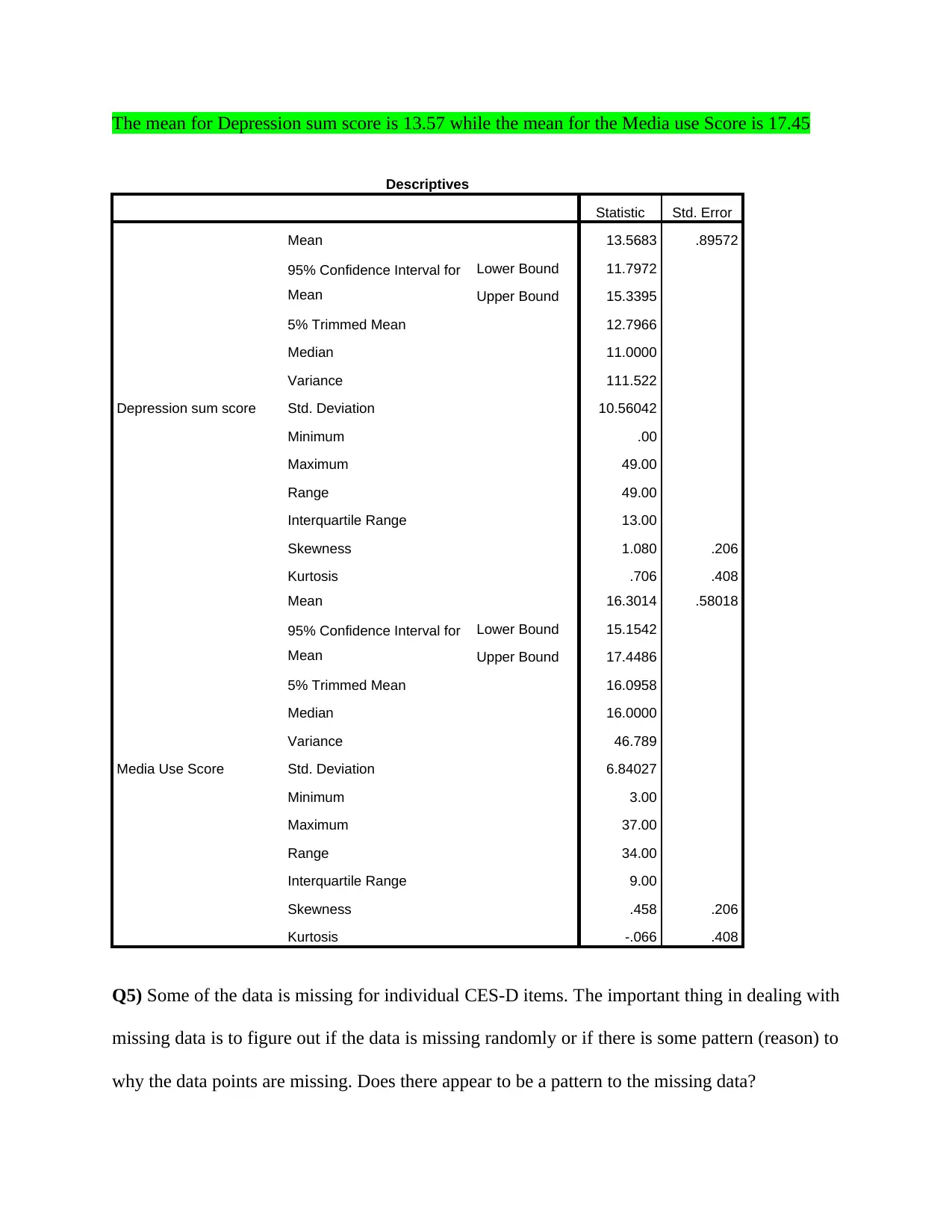
The mean for Depression sum score is 13.57 while the mean for the Media use Score is 17.45
Descriptives
Statistic Std. Error
Depression sum score
Mean 13.5683 .89572
95% Confidence Interval for
Mean
Lower Bound 11.7972
Upper Bound 15.3395
5% Trimmed Mean 12.7966
Median 11.0000
Variance 111.522
Std. Deviation 10.56042
Minimum .00
Maximum 49.00
Range 49.00
Interquartile Range 13.00
Skewness 1.080 .206
Kurtosis .706 .408
Media Use Score
Mean 16.3014 .58018
95% Confidence Interval for
Mean
Lower Bound 15.1542
Upper Bound 17.4486
5% Trimmed Mean 16.0958
Median 16.0000
Variance 46.789
Std. Deviation 6.84027
Minimum 3.00
Maximum 37.00
Range 34.00
Interquartile Range 9.00
Skewness .458 .206
Kurtosis -.066 .408
Q5) Some of the data is missing for individual CES-D items. The important thing in dealing with
missing data is to figure out if the data is missing randomly or if there is some pattern (reason) to
why the data points are missing. Does there appear to be a pattern to the missing data?

How might one deal with the missing data? (Do not do this, simply report what you think based
on our discussion this week).
Answer
There is no pattern to the missing data but rather they appear to be missing at random. Missing
data might be dealt with by removing the missing cases or doing imputation for the missing
cases.
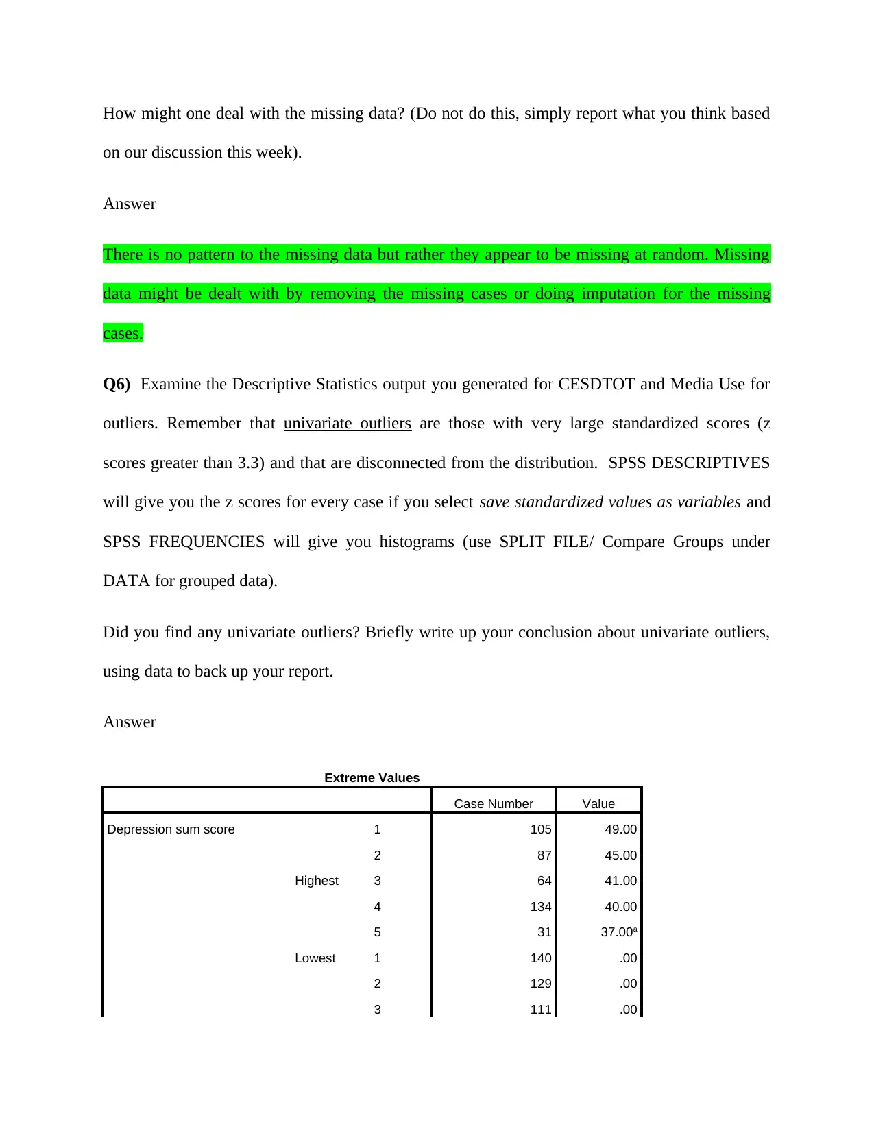
Q6) Examine the Descriptive Statistics output you generated for CESDTOT and Media Use for
outliers. Remember that univariate outliers are those with very large standardized scores (z
scores greater than 3.3) and that are disconnected from the distribution. SPSS DESCRIPTIVES
will give you the z scores for every case if you select save standardized values as variables and
SPSS FREQUENCIES will give you histograms (use SPLIT FILE/ Compare Groups under
DATA for grouped data).
Did you find any univariate outliers? Briefly write up your conclusion about univariate outliers,
using data to back up your report.
Answer
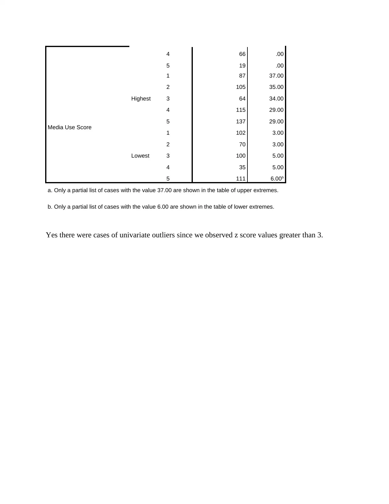
Extreme Values
Case Number Value
Depression sum score
Highest
1 105 49.00
2 87 45.00
3 64 41.00
4 134 40.00
5 31 37.00a
Lowest 1 140 .00
2 129 .00
3 111 .00

4 66 .00
5 19 .00
Media Use Score
Highest
1 87 37.00
2 105 35.00
3 64 34.00
4 115 29.00
5 137 29.00
Lowest
1 102 3.00
2 70 3.00
3 100 5.00
4 35 5.00
5 111 6.00b
a. Only a partial list of cases with the value 37.00 are shown in the table of upper extremes.
b. Only a partial list of cases with the value 6.00 are shown in the table of lower extremes.
Yes there were cases of univariate outliers since we observed z score values greater than 3.

Q7) Finally, write up the results of your descriptive statistics analysis (Q1-6) in APA format as
if you were describing the analysis for your dissertation (it will probably be only a paragraph).
Make sure to include figures (e.g., a box plot). The APA formatting may be difficult, but it will
be helpful in the long run to spend some time learning it properly now.
Answer
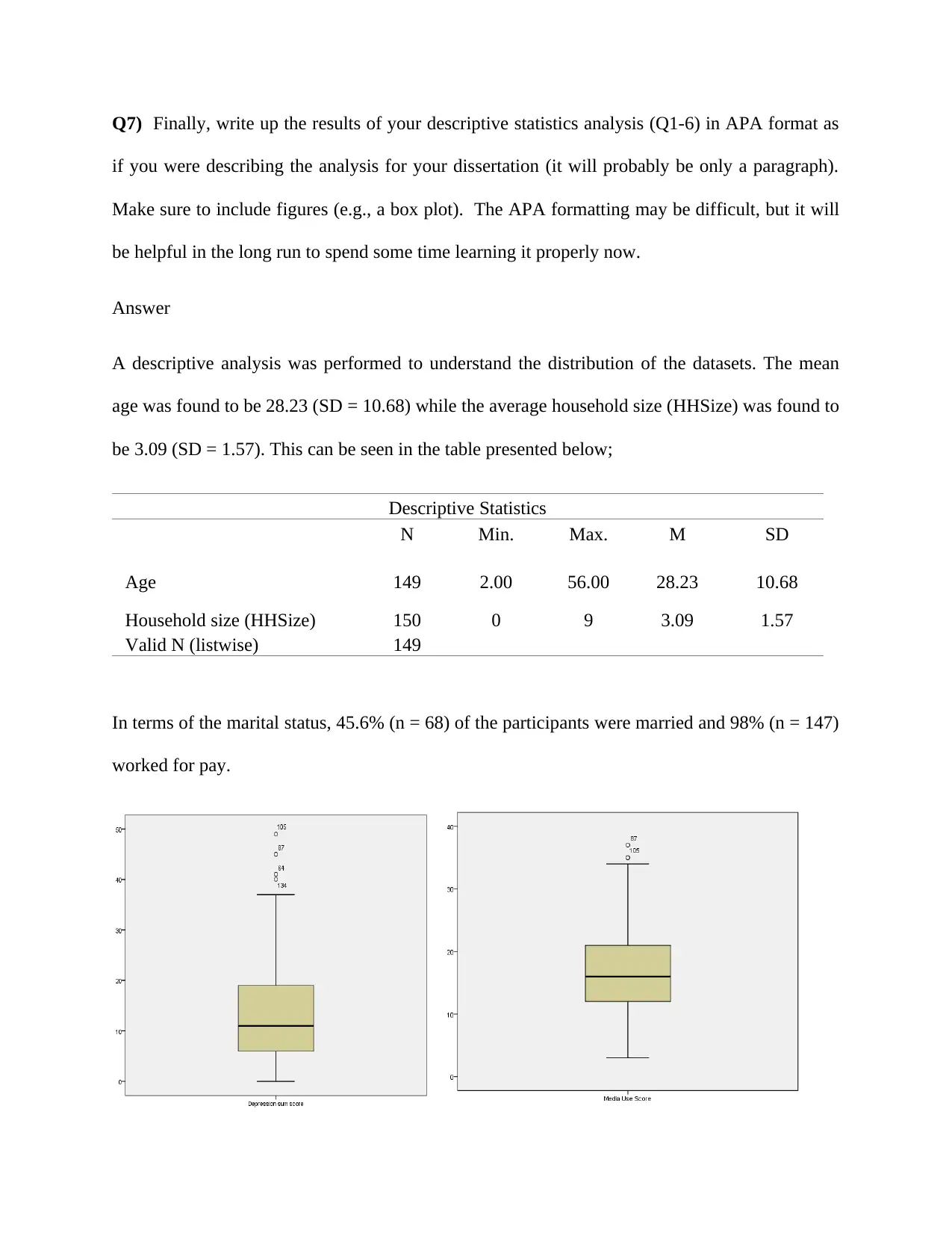
A descriptive analysis was performed to understand the distribution of the datasets. The mean
age was found to be 28.23 (SD = 10.68) while the average household size (HHSize) was found to
be 3.09 (SD = 1.57). This can be seen in the table presented below;
Descriptive Statistics
N Min. Max. M SD
Age 149 2.00 56.00 28.23 10.68
Household size (HHSize) 150 0 9 3.09 1.57
Valid N (listwise) 149
In terms of the marital status, 45.6% (n = 68) of the participants were married and 98% (n = 147)
worked for pay.

From the boxplots constructed, the plots revealed that outliers were present in the Media use
score as well as the depression sum scores
There was however no pattern for the missing data but rather the data seemed to be missing at
random. The missing data were random for the various variables and not associated with say a
particular subject or particular item.
Part 2

Inferential Statistics
Paired T-test
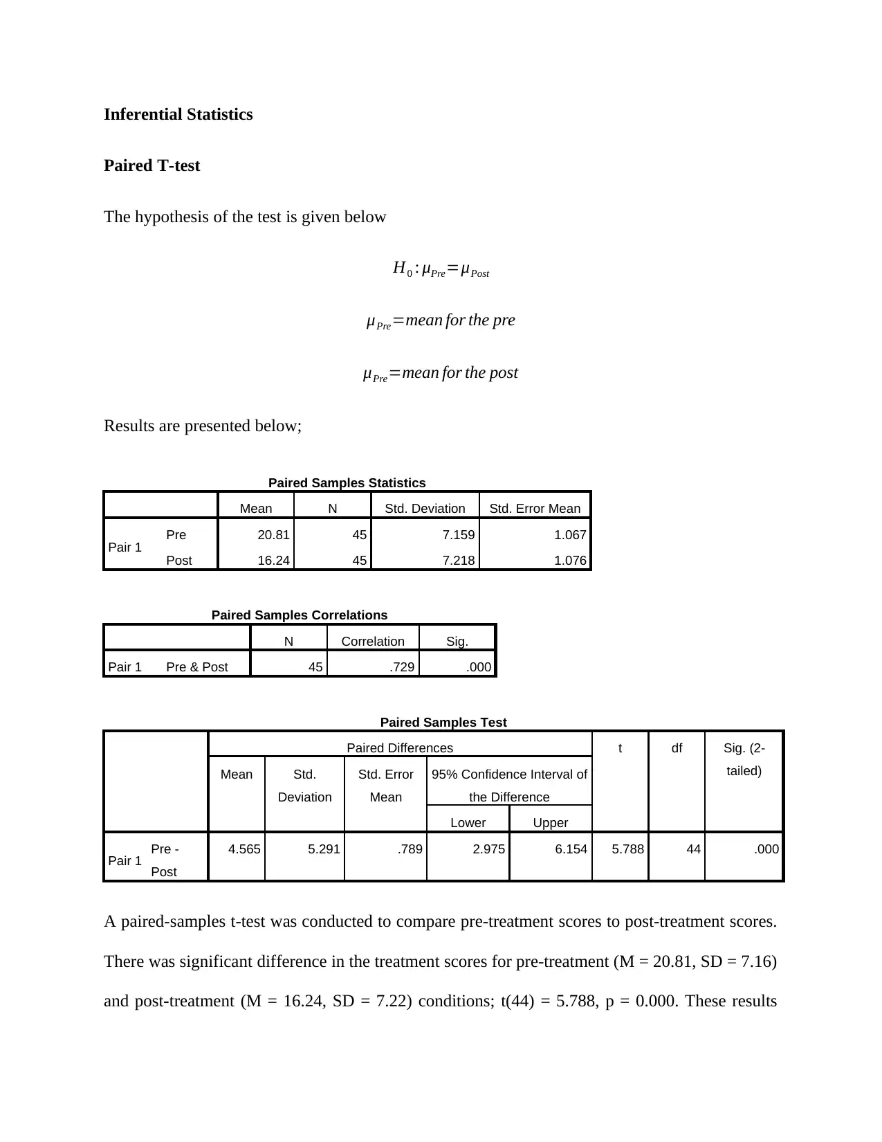
The hypothesis of the test is given below
H0 : μPre=μPost
μPre=mean for the pre
μPre=mean for the post
Results are presented below;
Paired Samples Statistics
Mean N Std. Deviation Std. Error Mean
Pair 1 Pre 20.81 45 7.159 1.067
Post 16.24 45 7.218 1.076
Paired Samples Correlations
N Correlation Sig.
Pair 1 Pre & Post 45 .729 .000
Paired Samples Test
Paired Differences t df Sig. (2-
tailed)Mean Std.
Deviation
Std. Error
Mean
95% Confidence Interval of
the Difference
Lower Upper
Pair 1 Pre -
Post
4.565 5.291 .789 2.975 6.154 5.788 44 .000
A paired-samples t-test was conducted to compare pre-treatment scores to post-treatment scores.
There was significant difference in the treatment scores for pre-treatment (M = 20.81, SD = 7.16)
and post-treatment (M = 16.24, SD = 7.22) conditions; t(44) = 5.788, p = 0.000. These results

suggest that there is a significant overall change between pre and post PTSD symptoms. The
overall treatment effect was quite significant in the sense that people get better over time.
ANOVA
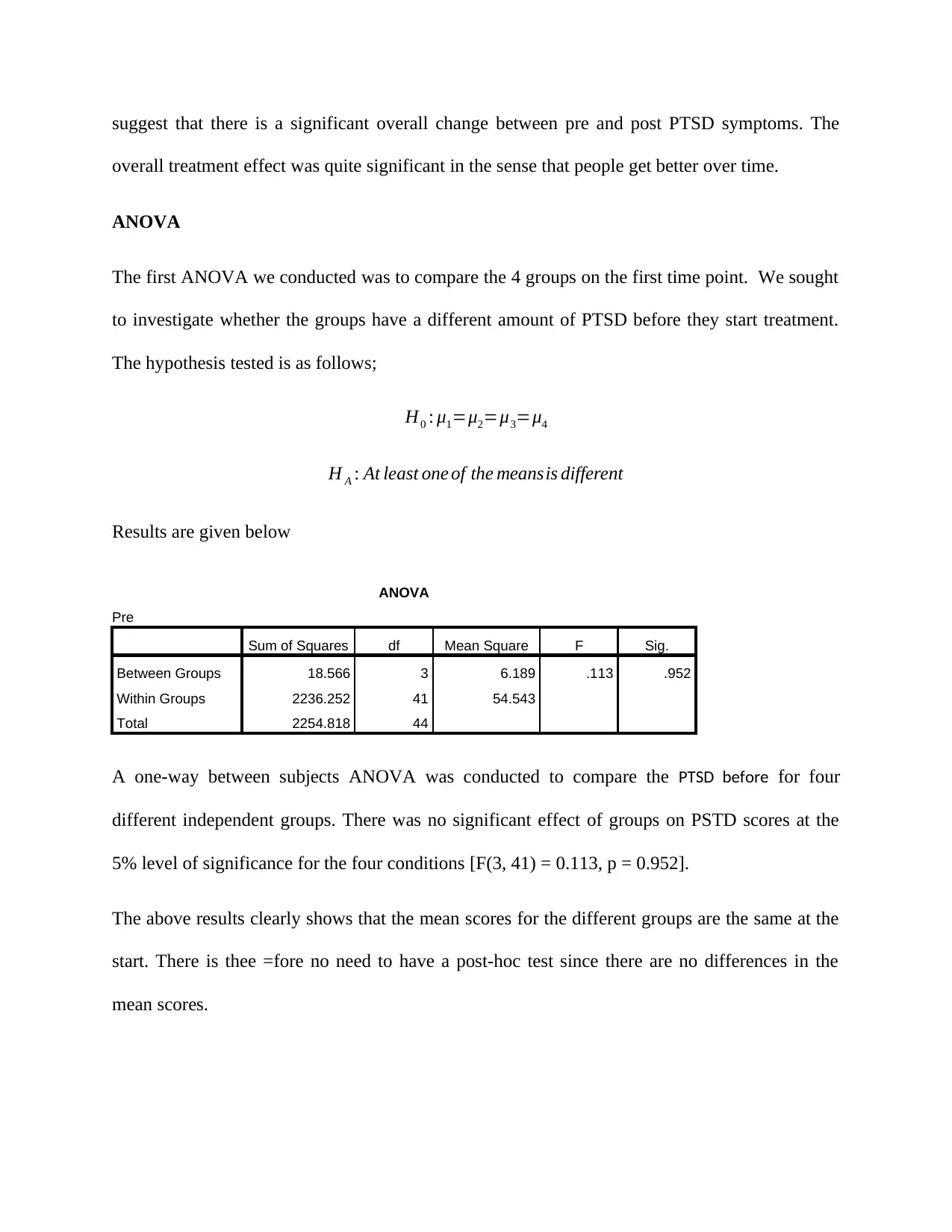
The first ANOVA we conducted was to compare the 4 groups on the first time point. We sought
to investigate whether the groups have a different amount of PTSD before they start treatment.
The hypothesis tested is as follows;
H0 : μ1=μ2=μ3=μ4
H A : At least one of the meansis different
Results are given below
ANOVA
Pre
Sum of Squares df Mean Square F Sig.
Between Groups 18.566 3 6.189 .113 .952
Within Groups 2236.252 41 54.543
Total 2254.818 44
A one-way between subjects ANOVA was conducted to compare the PTSD before for four
different independent groups. There was no significant effect of groups on PSTD scores at the
5% level of significance for the four conditions [F(3, 41) = 0.113, p = 0.952].
The above results clearly shows that the mean scores for the different groups are the same at the
start. There is thee =fore no need to have a post-hoc test since there are no differences in the
mean scores.

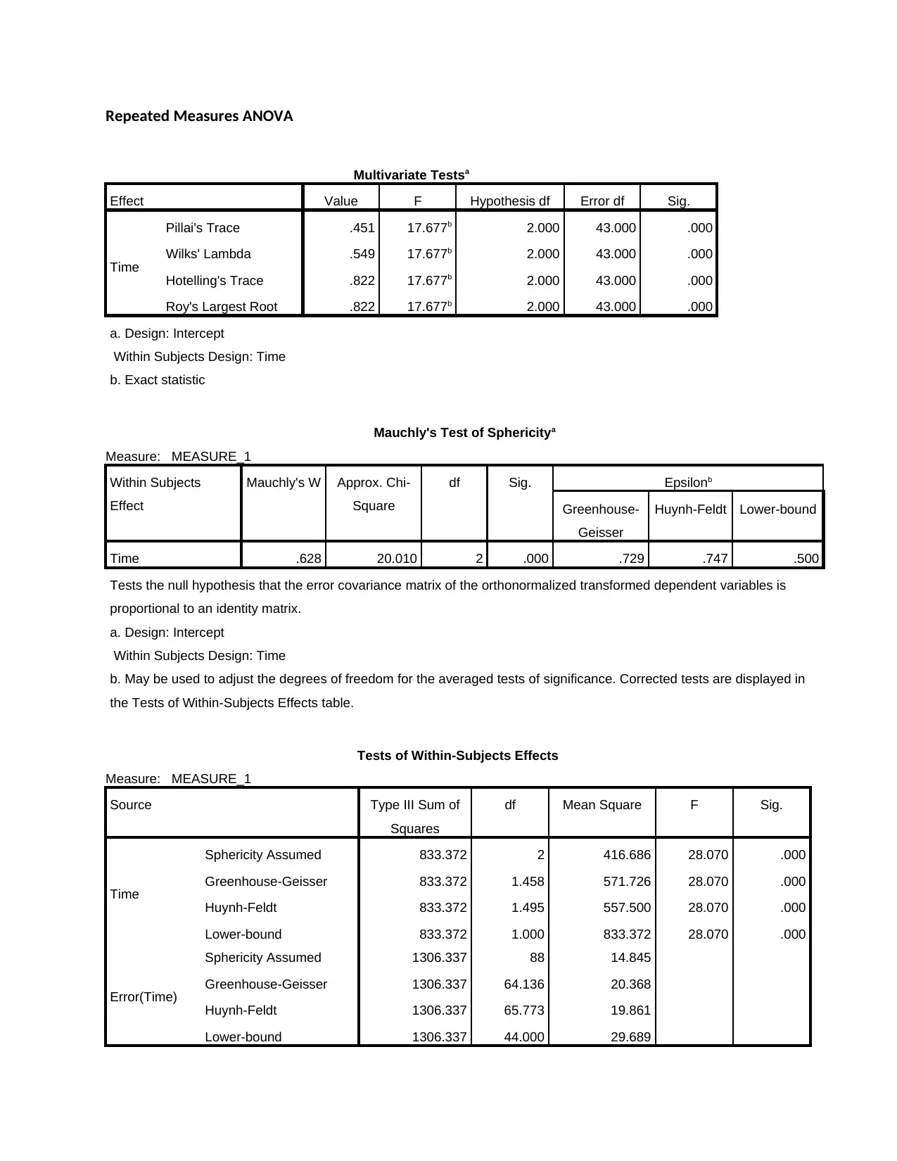
Repeated Measures ANOVA
Multivariate Testsa
Effect Value F Hypothesis df Error df Sig.
Time
Pillai's Trace .451 17.677b 2.000 43.000 .000
Wilks' Lambda .549 17.677b 2.000 43.000 .000
Hotelling's Trace .822 17.677b 2.000 43.000 .000
Roy's Largest Root .822 17.677b 2.000 43.000 .000
a. Design: Intercept
Within Subjects Design: Time
b. Exact statistic
Mauchly's Test of Sphericitya
Measure: MEASURE_1
Within Subjects
Effect
Mauchly's W Approx. Chi-
Square
df Sig. Epsilonb
Greenhouse-
Geisser
Huynh-Feldt Lower-bound
Time .628 20.010 2 .000 .729 .747 .500
Tests the null hypothesis that the error covariance matrix of the orthonormalized transformed dependent variables is
proportional to an identity matrix.
a. Design: Intercept
Within Subjects Design: Time
b. May be used to adjust the degrees of freedom for the averaged tests of significance. Corrected tests are displayed in
the Tests of Within-Subjects Effects table.
Tests of Within-Subjects Effects
Measure: MEASURE_1
Source Type III Sum of
Squares
df Mean Square F Sig.
Time
Sphericity Assumed 833.372 2 416.686 28.070 .000
Greenhouse-Geisser 833.372 1.458 571.726 28.070 .000
Huynh-Feldt 833.372 1.495 557.500 28.070 .000
Lower-bound 833.372 1.000 833.372 28.070 .000
Error(Time)
Sphericity Assumed 1306.337 88 14.845
Greenhouse-Geisser 1306.337 64.136 20.368
Huynh-Feldt 1306.337 65.773 19.861
Lower-bound 1306.337 44.000 29.689

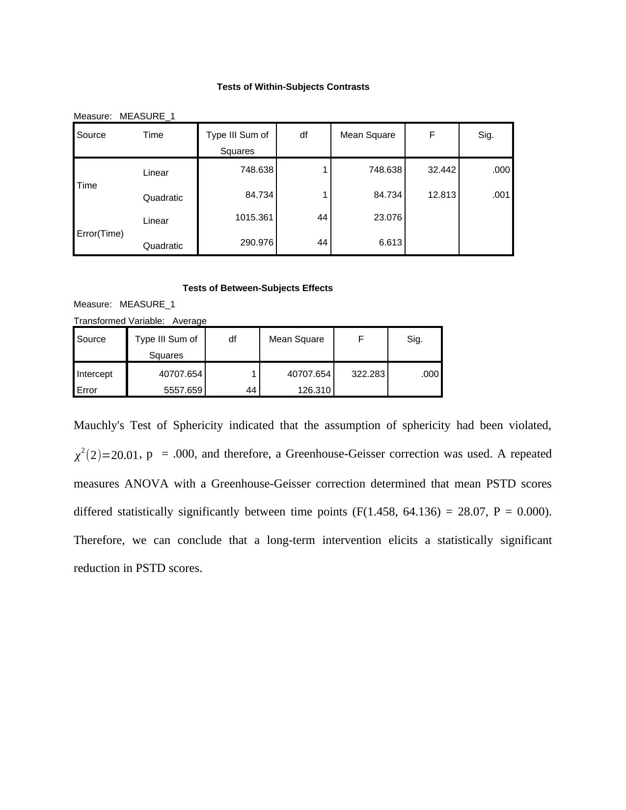
Tests of Within-Subjects Contrasts
Measure: MEASURE_1
Source Time Type III Sum of
Squares
df Mean Square F Sig.
Time
Linear 748.638 1 748.638 32.442 .000
Quadratic 84.734 1 84.734 12.813 .001
Error(Time)
Linear 1015.361 44 23.076
Quadratic 290.976 44 6.613
Tests of Between-Subjects Effects
Measure: MEASURE_1
Transformed Variable: Average
Source Type III Sum of
Squares
df Mean Square F Sig.
Intercept 40707.654 1 40707.654 322.283 .000
Error 5557.659 44 126.310
Mauchly's Test of Sphericity indicated that the assumption of sphericity had been violated,
χ2 (2)=20.01, p = .000, and therefore, a Greenhouse-Geisser correction was used. A repeated
measures ANOVA with a Greenhouse-Geisser correction determined that mean PSTD scores
differed statistically significantly between time points (F(1.458, 64.136) = 28.07, P = 0.000).
Therefore, we can conclude that a long-term intervention elicits a statistically significant
reduction in PSTD scores.

Repeated measures ANOVA
Multivariate Testsa
Effect Value F Hypothesis df Error df Sig.
Time
Pillai's Trace .525 22.088b 2.000 40.000 .000
Wilks' Lambda .475 22.088b 2.000 40.000 .000
Hotelling's Trace 1.104 22.088b 2.000 40.000 .000
Roy's Largest Root 1.104 22.088b 2.000 40.000 .000
Time * Group
Pillai's Trace .375 3.151 6.000 82.000 .008
Wilks' Lambda .647 3.247b 6.000 80.000 .007
Hotelling's Trace .513 3.335 6.000 78.000 .006
Roy's Largest Root .437 5.976c 3.000 41.000 .002
a. Design: Intercept + Group
Within Subjects Design: Time
b. Exact statistic
c. The statistic is an upper bound on F that yields a lower bound on the significance level.

Mauchly's Test of Sphericitya
Measure: MEASURE_1
Within Subjects
Effect
Mauchly's W Approx. Chi-
Square
df Sig. Epsilonb
Greenhouse-
Geisser
Huynh-Feldt Lower-bound
Time .714 13.488 2 .001 .777 .862 .500
Tests the null hypothesis that the error covariance matrix of the orthonormalized transformed dependent variables is
proportional to an identity matrix.
a. Design: Intercept + Group
Within Subjects Design: Time
b. May be used to adjust the degrees of freedom for the averaged tests of significance. Corrected tests are displayed in
the Tests of Within-Subjects Effects table.
Tests of Within-Subjects Effects
Measure: MEASURE_1
Source Type III Sum of
Squares
df Mean Square F Sig.
Time
Sphericity Assumed 778.949 2 389.474 32.412 .000
Greenhouse-Geisser 778.949 1.555 500.953 32.412 .000
Huynh-Feldt 778.949 1.723 452.034 32.412 .000
Lower-bound 778.949 1.000 778.949 32.412 .000
Time * Group
Sphericity Assumed 321.009 6 53.501 4.452 .001
Greenhouse-Geisser 321.009 4.665 68.815 4.452 .002
Huynh-Feldt 321.009 5.170 62.095 4.452 .001
Lower-bound 321.009 3.000 107.003 4.452 .008
Error(Time)
Sphericity Assumed 985.328 82 12.016
Greenhouse-Geisser 985.328 63.752 15.456
Huynh-Feldt 985.328 70.651 13.946
Lower-bound 985.328 41.000 24.032
Tests of Within-Subjects Contrasts
Measure: MEASURE_1
Source Time Type III Sum of
Squares
df Mean Square F Sig.
Time Linear 698.646 1 698.646 38.467 .000

Quadratic 80.303 1 80.303 13.680 .001
Time * Group Linear 270.703 3 90.234 4.968 .005
Quadratic 50.306 3 16.769 2.857 .049
Error(Time) Linear 744.658 41 18.162
Quadratic 240.670 41 5.870
Tests of Between-Subjects Effects
Measure: MEASURE_1
Transformed Variable: Average
Source Type III Sum of
Squares
df Mean Square F Sig.
Intercept 40618.546 1 40618.546 331.760 .000
Group 537.877 3 179.292 1.464 .238
Error 5019.782 41 122.434

Part 3
1. Open the data file (called RSM801Week3.sav). Explore the data file. Note, you will
not analyze all of these variables. Try to find the variables that are relevant to the
study description above. Write the names of the two variables here:
Answer
The variables are voter intention index and Ebola search volume index
2. Run a correlation analysis to test if there is an association between the Ebola search
volume index and the voter intention index. A correlation coefficient indicates the
strength and direction of a relationship between two variables. (select Analyze –
correlate – bivariate). Be sure to check off Options – Means and standard deviations.
In SPSS, be sure to check the box of the correct correlation type (Pearson, Spearman
or Kendall’s tau-b) for this data. Indicate the correlation type and why this is the
right choice for these variables:
Answer
Correlation Type: Pearson Correlation
Why: Because the data is an interval scale
Correlations
Voter Intention
Index
Ebola Search
Volume Index
Voter Intention Index
Pearson Correlation 1 .505*
Sig. (2-tailed) .012
N 24 24
Ebola Search Volume Index
Pearson Correlation .505* 1
Sig. (2-tailed) .012
N 24 65

*. Correlation is significant at the 0.05 level (2-tailed).
3. Write an APA formatted sentence describing the mean and standard deviation for
these two variables.
Answer
The average voter intention index was 1.12 (SD = 0.89) while the average Ebola
search volume index was 24.17 (SD = 22.85).
Descriptive Statistics
N Minimum Maximum Mean Std. Deviation
Voter Intention Index 24 -.40 2.40 1.1167 .88596
Ebola Search Volume Index 65 2.86 70.86 24.1712 22.84665
Valid N (listwise) 24
4. Report the results of the correlation in an APA statement (e.g., r (N-2) = .xx, p = .yyy.
Be sure to include degrees of freedom and statistical significance.
Answer
The two variables had a moderate positive relation, r(24) = .49, p = 0.012.
5. Write a sentence interpreting what these findings mean. That is, following periods
characterized by especially heavy periods of Ebola related Internet search activity,
was this search activity related or unrelated to voting intentions? If related, were U.S.
voters more likely to vote for a Republican or Democrat candidate? Does the
relationship appear to be direct (i.e., positive) or inverse (i.e, negative)?
Answer
Results showed that there is a significant positive relationship between voter intention
index and Ebola search volume index. This means that an increase in the Ebola search

volume index would result to an increase in voter intention index. On the other hand a
decrease in Ebola search volume index would result to a subsequent decrease in voter
intention index
[AFTER ANSWERING Q5, CONTINUE ON TO NEXT PAGE FOR Q’s 6 – 16]
6. [This question is optional extra credit] Next, to test whether the association between
these variables is stronger during the period just prior to and after the Ebola outbreak,
select only the scores from the two-week period including the last week of September
and the first week of October (use Data – Select Cases – If Condition is Satisfied,
specifying the condition (1) that would meet this criteria). Re-run the correlation
analyses for the association between Ebola search volume index and voter intention
index. Also, compute the correlation analysis between Daily Ebola search volume and
voter intention index. Which correlation value was stronger? Write an APA statement
summarizing these results.
Answer
Correlations
Voter Intention
Index
Ebola Search
Volume Index
Daily Ebola
Search Volume
Voter Intention Index
Pearson Correlation 1 .988** .607
Sig. (2-tailed) .000 .111
N 8 8 8
Ebola Search Volume Index
Pearson Correlation .988** 1 .693**
Sig. (2-tailed) .000 .006
N 8 14 14
Daily Ebola Search Volume
Pearson Correlation .607 .693** 1
Sig. (2-tailed) .111 .006
N 8 14 14
**. Correlation is significant at the 0.01 level (2-tailed).

A Pearson correlation test was performed to check the relationship between Ebola search volume
index and Daily Ebola search volume with the Voter intention index during the period just prior
to and after the Ebola outbreak. Results showed that a very strong positive relationship between
Voter intention index and Ebola search volume index, r(8) = 0.988, p = 0.000. A strong positive
but insignificant relationship was observed between Voter intention index and Daily Ebola
search volume, r(8) = 0.607, p = 0.111.
Correlation value was stronger between voter intention index and Ebola search volume index.
7. Make sure that all the data is selected (i.e., that the Select cases is set to “All Cases”).
Run a correlational analysis between ALL of the scale variables.
Which one is the strongest pair?
Which pair has the weakest relationship?
Correlations
Voter Intention
Index
Ebola Search
Volume Index
Daily Ebola
Search Volume
Voter Intention Index
Pearson Correlation 1 .505* .169
Sig. (2-tailed) .012 .430
N 24 24 24
Ebola Search Volume Index
Pearson Correlation .505* 1 .831**
Sig. (2-tailed) .012 .000
N 24 65 65
Daily Ebola Search Volume
Pearson Correlation .169 .831** 1
Sig. (2-tailed) .430 .000
N 24 65 65
*. Correlation is significant at the 0.05 level (2-tailed).
**. Correlation is significant at the 0.01 level (2-tailed).
The stronger pair is between Voter intention index and Ebola Search volume index
The pair with weak relationship is between Voter intention index and Daily Ebola Search
volume.

8. Prepare a series of scatterplots (making sure to follow APA-style guidelines). Select
Graphs – Chart Builder and then choose “Scatter/Dot” as the chart type. First, depict
the relationship between day and the voter intention index for the month of
September (demonstrating the relationship for voter intention index for the month
prior to the Ebola outbreak was announced). Please note that you will need to change
the select function as you did in Question 6 (but this time using the variable month,
selecting September as the month). Include the figure (formatting with an APA style
title) and write a sentence describing the relationship.
Answer
A negative relationship was observed between voter intention index for the month prior to
the Ebola outbreak was announced and the daily Ebola search volume.

9. Second, depict the relationship between day and the voter intention index for the last
week of September (i.e., the week prior to the outbreak was announced, Sept 24-30).
Include the figure (formatting with an APA style title) and write a sentence describing
the relationship.
Answer
A positive relationship was observed between voter intention index for the last week of
September and the daily Ebola search volume.

10. Third, depict the relationship between day and the voter intention index for the month
of October (i.e., the month after the outbreak was announced). Include the figure
(formatting with an APA style title) and write a sentence describing the relationship.
Answer
A negative relationship was observed between voter intention index for index for the month of
October and the daily Ebola search volume.
11. Finally, depict the relationship between day and the voter intention index for the first
week of October (i.e., 10/1-10/7, the week after the Ebola outbreak was announced).
Include the figure (formatting with an APA style title) and write a sentence describing
the relationship.
Answer

A positive relationship was observed between voter intention index for the first week of
October and the daily Ebola search volume.
12. Does viewing these graphs influence your interpretation of the correlation analyses
above? How so?
Answer
Yes viewing these graphs influence my interpretation of the correlation analyses
above. This is because daily Ebola search volume influences voter intention index
differently depending on the period when the Ebola was announced.
13. Conduct a t-test on voter intention index to assess whether voter intentions differed
whether they were expressed before (group = 1) or after (group = 2) the initial Ebola
outbreak was announced (Variable: newmonth). Based on this data, put a check in
front of the type of t-test you should carry out (and carry it out, using the Pace book
and/or notes from RSM701).

Answer
Independent sample t-test
Group Statistics
Two.weeks.prior.to.outbrea
k.only
N Mean Std. Deviation Std. Error Mean
Voter Intention Index Not in the 2 week window 16 1.5750 .62450 .15612
Within 2 week window 8 .2000 .55032 .19457
Independent Samples Test
Levene's Test for
Equality of
Variances
t-test for Equality of Means
F Sig. t df Sig. (2-
tailed)
Mean
Differen
ce
Std.
Error
Differen
ce
95% Confidence
Interval of the
Difference
Lower Upper
Voter Intention
Index
Equal variances
assumed
.167 .687 5.276 22 .000 1.37500 .26063 .83449 1.91551
Equal variances
not assumed
5.512 15.850 .000 1.37500 .24946 .84575 1.90425
14. Examining your output, write a sentence reporting the mean support for Republican
(relative to democratic) candidates for the Month prior to the outbreak as well as
proceeding the outbreak. Please be sure to use terms such as more, less, or about the
same to indicate whether support was greater prior to or after the outbreak was
announced.
Answer
The mean support for Republican (relative to democratic) candidates for the Month
prior to the outbreak as well as proceeding the outbreak was more than during the

outbreak period. His shows that support was greater prior to or after the outbreak was
announced
15. Assess whether this change was statistically significant. Write an APA statement
with the t-test findings (e.g., t (df) = xx.xx, p = .yyy). Don’t forget to use the
Levene’s test to determine whether you should be reporting the row of findings that
consider “equal variances assumed” (when Levene’s test p > .05) or equal variances
not assumed (when Levene’s test p < .05). Interpret this finding.
Answer
An independent samples t-test was performed to compare the average voter intention
index. The Levene’s test showed that we assume equal variances (p-value < 0.05).
Results showed that the average voter intention index Not in the 2 week window (M
= 1.58, SD = 0.62, N = 12) was significant different with the average voter intention
index within 2 week window (M = 0.20, SD = 0.55, N = 8), t (22) = 5.276, p < .05,
two-tailed. The difference of 1.375 showed a significant difference. Essentially
results showed that Ebola outbreak did significantly reduce the voter intention index
16. What does the t-test tell you? What does the correlation tell you? How are each useful
to understanding this data?
Answer
T-test tells us the difference in the average voter intention index for the two time
points while correlation tells us the relationship that exists between the voter intention
index and daily Ebola search volume. The two tests are important since they are able
to tell us the relationship that the different factors have on the voter intention index.