FIN200 Assignment: Capital Market Line, Security Market Line, and CAPM
VerifiedAdded on 2023/06/07
|11
|2645
|455
Report
AI Summary
This report provides a comprehensive analysis of key concepts in finance, focusing on the Capital Market Line (CML) and the Security Market Line (SML) within the context of the Capital Asset Pricing Model (CAPM). It elucidates the differences between CML and SML, emphasizing their roles in assessing portfolio efficiency and risk-return balance. The report delves into the concept of minimum variance portfolios, explaining their significance in diversifying investments to reduce overall portfolio risk. Furthermore, it examines the relevance of the CAPM equation in determining the required rate of return, highlighting its importance in investment appraisal. The report includes graphical representations and equations for clarity, and it concludes by summarizing the importance of these financial tools for investors. The assignment is structured to demonstrate an understanding of portfolio optimization, risk management, and the application of financial models in investment decision-making.

FIN200 Assignment, Trimester 2 2018
Paraphrase This Document
Need a fresh take? Get an instant paraphrase of this document with our AI Paraphraser
TABLE OF CONTENTS
Introduction......................................................................................................................................3
Difference between CML and SML................................................................................................3
Assessment of capital market line and security market line........................................................3
Graphical representation of the security market line...................................................................5
Minimum variance portfolio........................................................................................................7
The relevance of the equation of capital asset pricing model......................................................8
Conclusion.......................................................................................................................................9
References......................................................................................................................................10
INTRODUCTION
The optimum portfolio is that in which the investor get a high return, but for building the optimal
portfolio the risk factor of the investment is a very important aspect which is to be considered.
The risk factor of the asset depends on the attitude of the investor towards their risk-bearing
capacity (Sinha, Chandwani and Sinha, 2015). Investors have different risk behaviour capacity
therefore by combining a different combination of securities they select the portfolio various
tools are applied. The present study emphasis on the difference between capital market line and
security market line for assessment of the efficiency of the developed portfolio by the investor.
Further, it evaluates the capital assets pricing model in terms of assessing the efficiency of the
risk and return of the portfolio so that investor can get maximum return on their investment.
Along with this, in this study minimum portfolio variance strategy is also analyzed by
considering suitable concepts.
DIFFERENCE BETWEEN CML AND SML
Assessment of capital market line and security market line
In capital assets pricing model, the capital market line showed the balance between the risk and
provided a return by the portfolio for achieving the efficient portfolio for the investor (Williams
and Dobelman, 2017). In this method, the position at the risk-free rate for the borrowings as well
as lending is selected by the investor, by which the maximum return on the existing risk, can be
achieved.
Graphical representation of Capital market line
⊘ This is a preview!⊘
Do you want full access?
Subscribe today to unlock all pages.
Trusted by 1+ million students worldwide
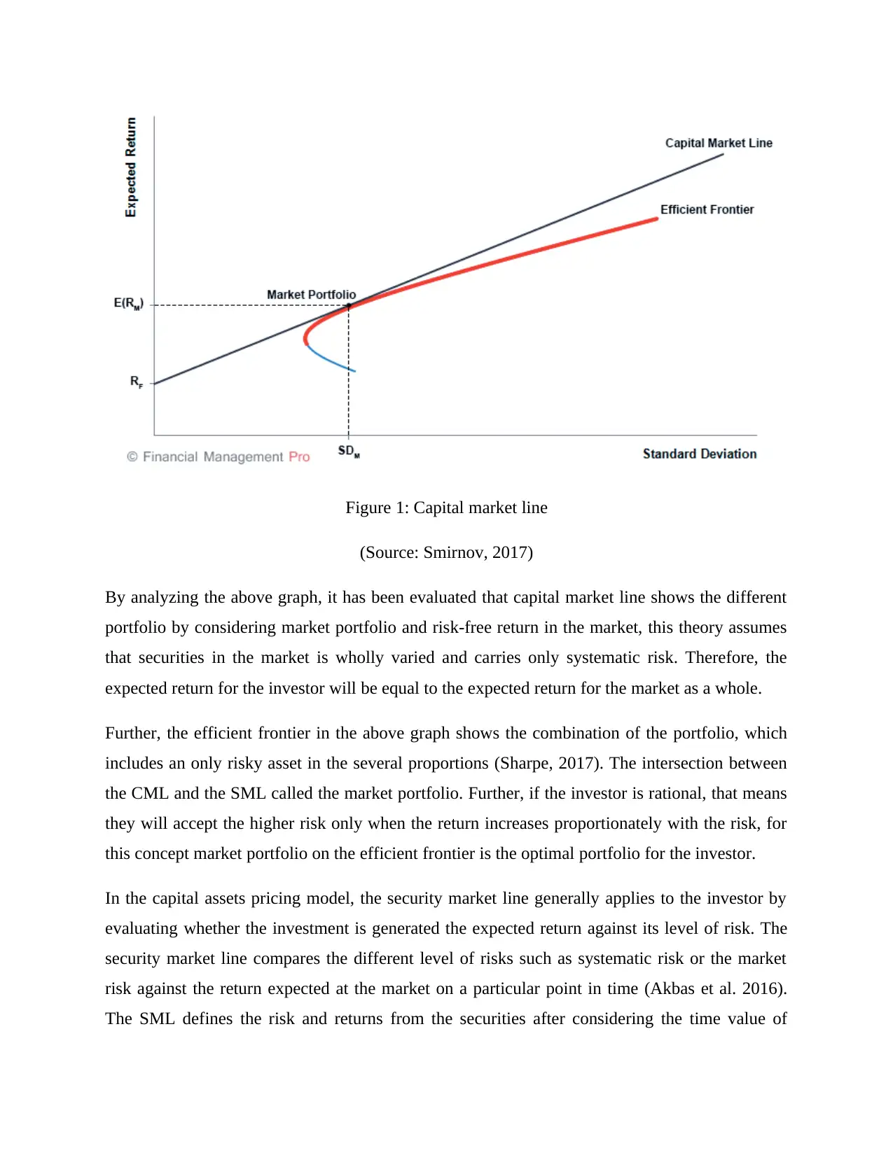
Figure 1: Capital market line
(Source: Smirnov, 2017)
By analyzing the above graph, it has been evaluated that capital market line shows the different
portfolio by considering market portfolio and risk-free return in the market, this theory assumes
that securities in the market is wholly varied and carries only systematic risk. Therefore, the
expected return for the investor will be equal to the expected return for the market as a whole.
Further, the efficient frontier in the above graph shows the combination of the portfolio, which
includes an only risky asset in the several proportions (Sharpe, 2017). The intersection between
the CML and the SML called the market portfolio. Further, if the investor is rational, that means
they will accept the higher risk only when the return increases proportionately with the risk, for
this concept market portfolio on the efficient frontier is the optimal portfolio for the investor.
In the capital assets pricing model, the security market line generally applies to the investor by
evaluating whether the investment is generated the expected return against its level of risk. The
security market line compares the different level of risks such as systematic risk or the market
risk against the return expected at the market on a particular point in time (Akbas et al. 2016).
The SML defines the risk and returns from the securities after considering the time value of
Paraphrase This Document
Need a fresh take? Get an instant paraphrase of this document with our AI Paraphraser
money and the risk premium. This concept of the security market line depicts that the investor
must get the compensation for the time value of the money and also the level of risk which is
accepted by the investor on their investment.
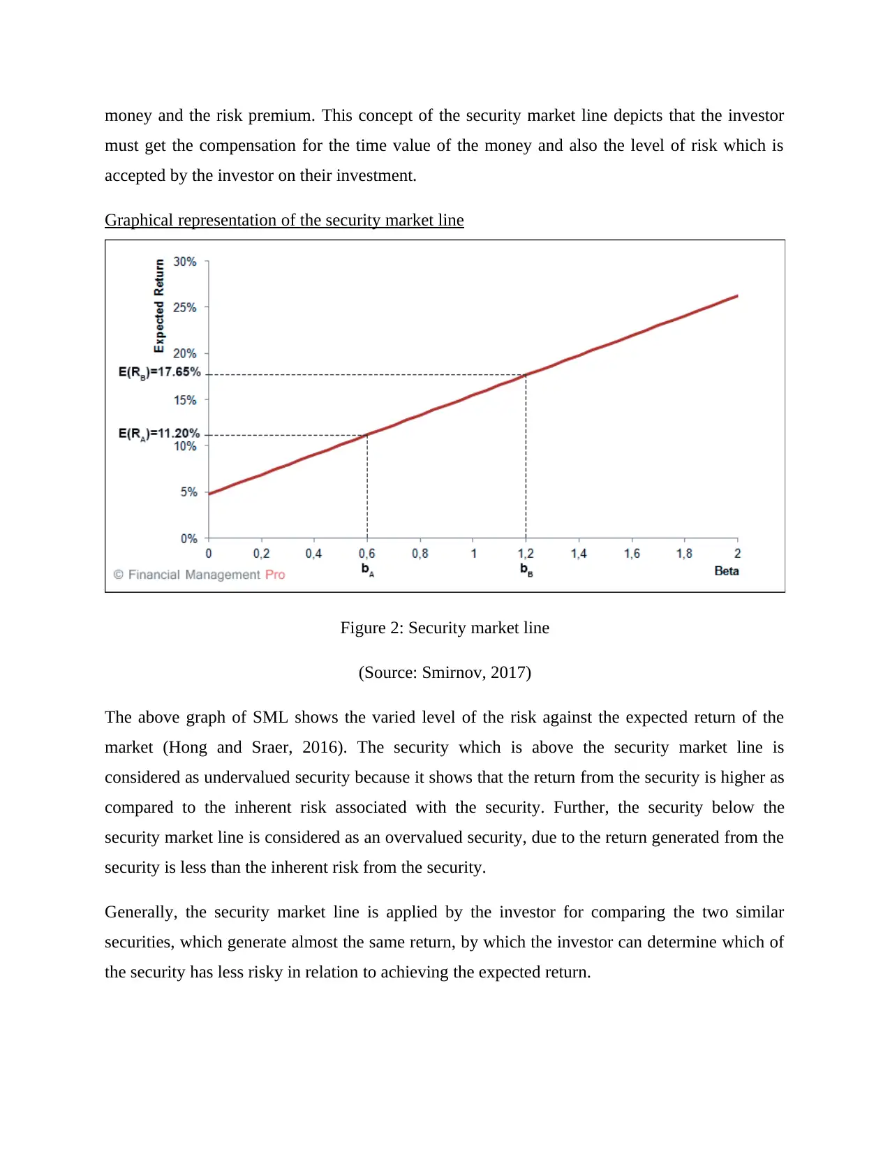
Graphical representation of the security market line
Figure 2: Security market line
(Source: Smirnov, 2017)
The above graph of SML shows the varied level of the risk against the expected return of the
market (Hong and Sraer, 2016). The security which is above the security market line is
considered as undervalued security because it shows that the return from the security is higher as
compared to the inherent risk associated with the security. Further, the security below the
security market line is considered as an overvalued security, due to the return generated from the
security is less than the inherent risk from the security.
Generally, the security market line is applied by the investor for comparing the two similar
securities, which generate almost the same return, by which the investor can determine which of
the security has less risky in relation to achieving the expected return.
must get the compensation for the time value of the money and also the level of risk which is
accepted by the investor on their investment.
Graphical representation of the security market line
Figure 2: Security market line
(Source: Smirnov, 2017)
The above graph of SML shows the varied level of the risk against the expected return of the
market (Hong and Sraer, 2016). The security which is above the security market line is
considered as undervalued security because it shows that the return from the security is higher as
compared to the inherent risk associated with the security. Further, the security below the
security market line is considered as an overvalued security, due to the return generated from the
security is less than the inherent risk from the security.
Generally, the security market line is applied by the investor for comparing the two similar
securities, which generate almost the same return, by which the investor can determine which of
the security has less risky in relation to achieving the expected return.
Therefore on the basis of the above study, it has been seen that although the CML and the SML
are applied in the context on the capital asset pricing model, both measures the risk and return of
the portfolio by applying some different parameters (Jylhä, 2018). The capital market line uses
the risk-free rate, and the associated risk of the particular portfolio to calculate the required
return on the portfolio, while the SML shows the varied level of the risk against the expected
return of the market as a whole on that particular point of time. Further, both the concepts are
applied by the investor to find out the risk associated with the investment, but the risk is
measured by CML through the standard deviation of the security, on the other hand, SML
measures the risk through the beta coefficient of the security. The graphical representation of the
CML shows the efficient frontier, by which the efficient portfolio of the security can be
evaluated, while the graphical representation of the security market line shows the both efficient
and the non-efficient portfolio. Moreover, the capital market line ascertained the market portfolio
and the risk-free asset while the security market line ascertained all the factors of the security.
The CML measures the risk and return of the efficient portfolio while the SML measures the risk
and return for the individual shares in the market. Further for measuring the risk factors of the
security implementation of the CML is regarded well than the SML.
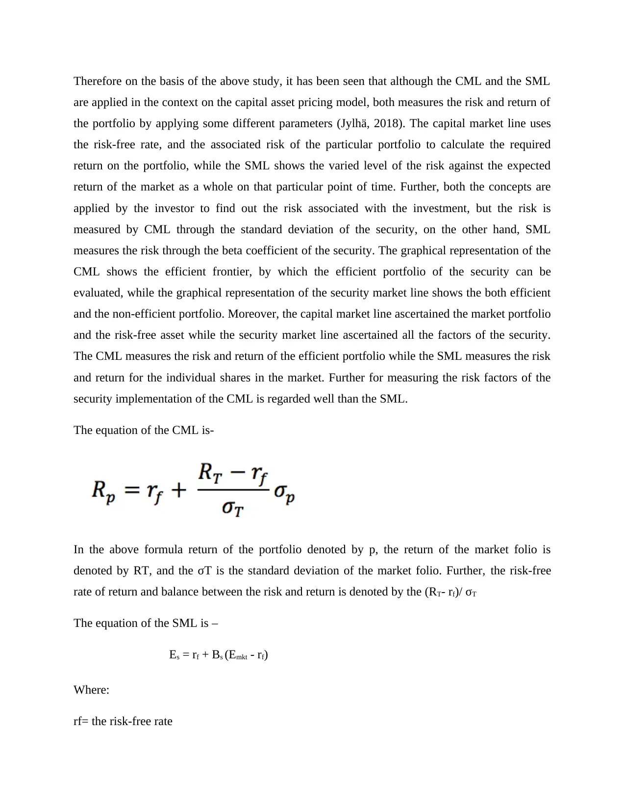
The equation of the CML is-
In the above formula return of the portfolio denoted by p, the return of the market folio is
denoted by RT, and the σT is the standard deviation of the market folio. Further, the risk-free
rate of return and balance between the risk and return is denoted by the (RT- rf)/ σT
The equation of the SML is –
Es = rf + Bs (Emkt - rf)
Where:
rf= the risk-free rate
are applied in the context on the capital asset pricing model, both measures the risk and return of
the portfolio by applying some different parameters (Jylhä, 2018). The capital market line uses
the risk-free rate, and the associated risk of the particular portfolio to calculate the required
return on the portfolio, while the SML shows the varied level of the risk against the expected
return of the market as a whole on that particular point of time. Further, both the concepts are
applied by the investor to find out the risk associated with the investment, but the risk is
measured by CML through the standard deviation of the security, on the other hand, SML
measures the risk through the beta coefficient of the security. The graphical representation of the
CML shows the efficient frontier, by which the efficient portfolio of the security can be
evaluated, while the graphical representation of the security market line shows the both efficient
and the non-efficient portfolio. Moreover, the capital market line ascertained the market portfolio
and the risk-free asset while the security market line ascertained all the factors of the security.
The CML measures the risk and return of the efficient portfolio while the SML measures the risk
and return for the individual shares in the market. Further for measuring the risk factors of the
security implementation of the CML is regarded well than the SML.
The equation of the CML is-
In the above formula return of the portfolio denoted by p, the return of the market folio is
denoted by RT, and the σT is the standard deviation of the market folio. Further, the risk-free
rate of return and balance between the risk and return is denoted by the (RT- rf)/ σT
The equation of the SML is –
Es = rf + Bs (Emkt - rf)
Where:
rf= the risk-free rate
⊘ This is a preview!⊘
Do you want full access?
Subscribe today to unlock all pages.
Trusted by 1+ million students worldwide
Bs = the beta of the investment
Emkg = the expected return of the market
Es =the expected return on the investment
Therefore it has been concluded by the above evaluation both the capital market line, and the
security market line is the capital asset pricing model determine the balance between the risk and
return of the securities by considering the different aspect of the factors of the security.
Minimum variance portfolio
Minimum variance portfolio refers to that portfolio in which the individual asset is considered
risky, but while the asset is combined together with the results in the lower risk and the
anticipated return (Yen, 2015). In other words, minimum portfolio variance is the diversified
portfolio, which combines the securities for reducing the price volatility of the overall portfolio.
Generally, the portfolio means a set of the investment keep by the investor in one account or the
combination of the securities and account kept by one investor (Coqueret, 2015). For creating the
minimum variance portfolio, an investor is required to have a combination of low volatility
investment so that the market risk can be reduced as the high volatility leads to higher market
risk or the investor through the combination of volatile investment with low correlation with
each other can also build the minimum variance portfolio.
Minimum portfolio assists in assigning the weight to the individual security in such as manner by
which the risk of the overall portfolio can be minimized. Minimum portfolio variance does not
affect by the expected return of the security. It depicts the lowest risk portfolio among all risk
and returns portfolio from the efficient portfolio. Though the application of the minimum
portfolio variance, investor, determine the securities in which the investor want to invest along
with limitations, can obtain the estimate of the returns, volatility, correlations of the investable
securities , then by applying this estimation in the real world, the investor gets the reliable output
from the investment in the security (Yang, Couillet and McKay, 2015). Moreover, the
investment that has the low correlation is described as that security that performs differently at
the same market and the economic environment, the investor on the basis of the minimum
portfolio variance can diversify the portfolio in such a manner by which the volatility can be
Paraphrase This Document
Need a fresh take? Get an instant paraphrase of this document with our AI Paraphraser
reduced. For instance, minimum portfolio variance implements by the investor for investing in
the stock mutual fund and the bond mutual fund (Bodnar and Gupta, 2015). Since the relation
between the prices of the stock and the bond are converse, it means if the price of the particular
security is increasing then the bond price is definitely decreasing and vice versa, which leads that
between the price of the stock and the price of the bond very low correlation exist. So that by
application of the minimum portfolio variance strategy investor can combine investment types of
risky and non-risky asset, so that can achieve the high relative return without high risk.
The relevance of the equation of capital asset pricing model
The capital asset pricing model establishes the linear relationship between the systematic risk
and the required rate of return on the investment. In this model, Systematic risk can be defined
as a risk which affects the overall market, and the investment may be in the stock market
securities or in the operations of the business (Zabarankin, Pavlikov and Uryasev, 2014).
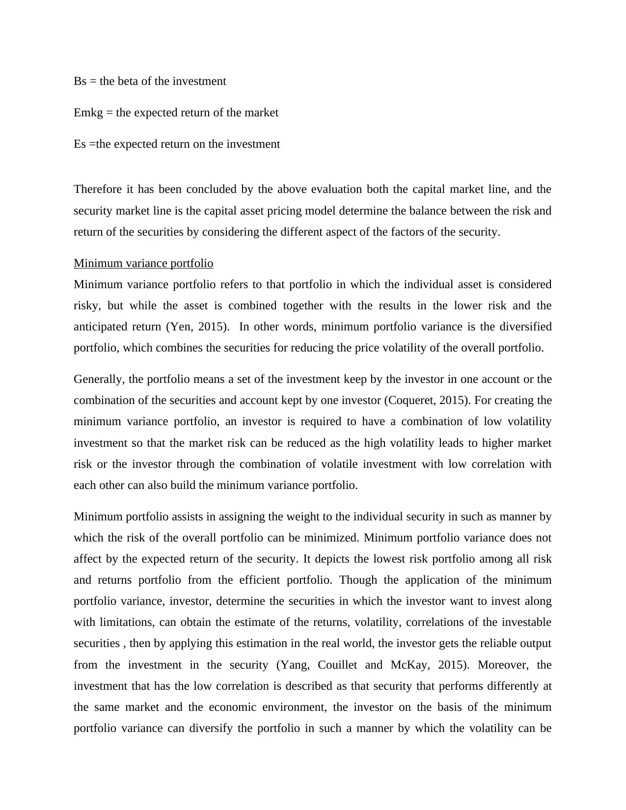
The equation of the CAPM is given below-
In this model, the assumption has been made that an investor should be compensated only for the
systematic risk in their portfolio because due to the diversification of the portfolio unsystematic
risk can be mitigated. Further, this model provides the discount rate better than any other pricing
model for the investment appraisal technique (Piamsuwannakit et al. 2015). Apart from the
above, this model also considers the systematic risk of the company is related to the overall risk
of the concerned market. CAPM equation suggests that investor should be earned for the time
value of money and the risk associated with their investment. Here the risk-free rate in the
equation depicts that investor should be compensated placing their investment in any investment
over the time along with this; it also shows that amount of the compensation required by the
the stock mutual fund and the bond mutual fund (Bodnar and Gupta, 2015). Since the relation
between the prices of the stock and the bond are converse, it means if the price of the particular
security is increasing then the bond price is definitely decreasing and vice versa, which leads that
between the price of the stock and the price of the bond very low correlation exist. So that by
application of the minimum portfolio variance strategy investor can combine investment types of
risky and non-risky asset, so that can achieve the high relative return without high risk.
The relevance of the equation of capital asset pricing model
The capital asset pricing model establishes the linear relationship between the systematic risk
and the required rate of return on the investment. In this model, Systematic risk can be defined
as a risk which affects the overall market, and the investment may be in the stock market
securities or in the operations of the business (Zabarankin, Pavlikov and Uryasev, 2014).
The equation of the CAPM is given below-
In this model, the assumption has been made that an investor should be compensated only for the
systematic risk in their portfolio because due to the diversification of the portfolio unsystematic
risk can be mitigated. Further, this model provides the discount rate better than any other pricing
model for the investment appraisal technique (Piamsuwannakit et al. 2015). Apart from the
above, this model also considers the systematic risk of the company is related to the overall risk
of the concerned market. CAPM equation suggests that investor should be earned for the time
value of money and the risk associated with their investment. Here the risk-free rate in the
equation depicts that investor should be compensated placing their investment in any investment
over the time along with this; it also shows that amount of the compensation required by the
investor for taking the additional risk. It can be measured by the return of the market over the
risk-free interest rate through the risk measure that is Beta of the security. Beta denotes the
volatility function of the market and the security along with the correlation between the security
and the market, by which the investor can get to know about the how risky is the asset as
compared to the overall market.
Due to the all above reason the equation of the capital asset pricing model more relevant than
other equation at the time of evaluating the return provided by the investment.
CONCLUSION
On the basis of the above study, it has been evaluated that CML and SML are the two technique
of the capital asset pricing model, by which the investor can assess their optimal portfolio.
However, the method of measuring the risk and return of the security can be done by both as
they consider different factors but have the same objectives. Further, the investor through the
minimum portfolio variance strategy can build the well-diversified portfolio by combining the
risky individual asset with the less risky asset, which leads to the maximum return on the
investment at the minimum risk. Apart from this, the capital asset pricing model is the best
method for determining the optimal portfolio, because the equation of the capital asset pricing
model considers various factor by which the risk and the return of the securities can be affected.
⊘ This is a preview!⊘
Do you want full access?
Subscribe today to unlock all pages.
Trusted by 1+ million students worldwide
REFERENCES
Akbas, F., Armstrong, W.J., Sorescu, S. and Subrahmanyam, A., 2016. Capital market efficiency
and arbitrage efficacy. Journal of Financial and Quantitative Analysis, 51(2), pp.387-413.
Bodnar, T. and Gupta, A.K., 2015. Robustness of the inference procedures for the global
minimum variance portfolio weights in a skew-normal model. The European Journal of
Finance, 21(13-14), pp.1176-1194.
Coqueret, G., 2015. Diversified minimum-variance portfolios. Annals of Finance, 11(2), pp.221-
241.
Hong, H. and Sraer, D.A., 2016. Speculative betas. The Journal of Finance, 71(5), pp.2095-
2144.
Jylhä, P., 2018. Margin requirements and the security market line. The Journal of
Finance, 73(3), pp.1281-1321.
Piamsuwannakit, S., Autchariyapanitkul, K., Sriboonchitta, S. and Ouncharoen, R., 2015,
October. Capital asset pricing model with interval data. In International Symposium on
Integrated Uncertainty in Knowledge Modelling and Decision Making (pp. 163-170). Springer,
Cham.
Sharpe, W., 2017. Capital Market Theory, Efficiency, and Imperfections. Quantitative Financial
Analytics: The Path to Investment Profits, p.445.
Sinha, P., Chandwani, A. and Sinha, T., 2015. Algorithm of construction of optimum portfolio of
stocks using genetic algorithm. International Journal of System Assurance Engineering and
Management, 6(4), pp.447-465.
Smirnov, Y., 2017. Capital Market Line – CML. [Online]. Available through <
http://financialmanagementpro.com/capital-market-line-cml/>. [Accessed on 17th September
2018].
Paraphrase This Document
Need a fresh take? Get an instant paraphrase of this document with our AI Paraphraser
Smirnov, Y., 2017. Security Market Line – SML. [Online]. Available through <
http://financialmanagementpro.com/security-market-line-sml/>. [Accessed on 17th September
2018].
Williams, E.E. and Dobelman, J.A., 2017. Capital Market Theory, Efficiency, and
Imperfections. World Scientific Book Chapters, pp.445-510.
Yang, L., Couillet, R. and McKay, M.R., 2015. A robust statistics approach to minimum
variance portfolio optimization. IEEE Transactions on Signal Processing, 63(24), pp.6684-6697.
Yen, Y.M., 2015. Sparse weighted-norm minimum variance portfolios. Review of
Finance, 20(3), pp.1259-1287.
Zabarankin, M., Pavlikov, K. and Uryasev, S., 2014. Capital asset pricing model (CAPM) with
drawdown measure. European Journal of Operational Research, 234(2), pp.508-517.
1 out of 11
Related Documents


Your All-in-One AI-Powered Toolkit for Academic Success.
+13062052269
info@desklib.com
Available 24*7 on WhatsApp / Email
![[object Object]](/_next/static/media/star-bottom.7253800d.svg)
Unlock your academic potential
Copyright © 2020–2025 A2Z Services. All Rights Reserved. Developed and managed by ZUCOL.