Financial Engineering Assignment: Bank RUPT TARF Product Solution

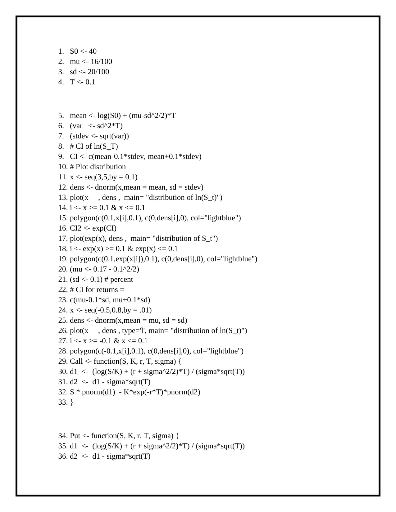
This document presents a comprehensive solution to a financial engineering take-home exam, focusing on the analysis of a Target Average Redemption Forward (TARF) product within the context of FX dynamics and derivatives. The assignment, set for a fictional bank named Bank RUPT, explores the modeling of exchange rates, specifically the CNY/USD pair, using a stochastic process. The solution encompasses various aspects of financial modeling, including the application of the Black-Scholes model, option pricing, and the calculation of confidence intervals. The student's work includes code, plots, and detailed explanations, addressing questions about the specification of FX dynamics, asset pricing under different measures, and the behavior of option prices with respect to various parameters. The solution also addresses the implicit volatility calculations and presents the evolution of stocks and calls, as well as stocks and puts, in percentage terms. The document provides a complete and detailed response to the assignment's questions and requirements, providing a good understanding of the concepts in financial engineering.

1. S0 <- 40
2. mu <- 16/100
3. sd <- 20/100
4. T <- 0.1
5. mean <- log(S0) + (mu-sd^2/2)*T
6. (var <- sd^2*T)
7. (stdev <- sqrt(var))
8. # CI of ln(S_T)
9. CI <- c(mean-0.1*stdev, mean+0.1*stdev)
10. # Plot distribution
11. x <- seq(3,5,by = 0.1)
12. dens <- dnorm(x,mean = mean, sd = stdev)
13. plot(x , dens , main= "distribution of ln(S_t)")
14. i <- x >= 0.1 & x <= 0.1
15. polygon(c(0.1,x[i],0.1), c(0,dens[i],0), col="lightblue")
16. CI2 <- exp(CI)
17. plot(exp(x), dens , main= "distribution of S_t")
18. i <- exp(x) >= 0.1 & exp(x) <= 0.1
19. polygon(c(0.1,exp(x[i]),0.1), c(0,dens[i],0), col="lightblue")
20. (mu <- 0.17 - 0.1^2/2)
21. (sd <- 0.1) # percent
22. # CI for returns =
23. c(mu-0.1*sd, mu+0.1*sd)
24. x <- seq(-0.5,0.8,by = .01)
25. dens <- dnorm(x,mean = mu, sd = sd)
26. plot(x , dens , type='l', main= "distribution of ln(S_t)")
27. i <- x >= -0.1 & x <= 0.1
28. polygon(c(-0.1,x[i],0.1), c(0,dens[i],0), col="lightblue")
29. Call <- function(S, K, r, T, sigma) {
30. d1 <- (log(S/K) + (r + sigma^2/2)*T) / (sigma*sqrt(T))
31. d2 <- d1 - sigma*sqrt(T)
32. S * pnorm(d1) - K*exp(-r*T)*pnorm(d2)
33. }
34. Put <- function(S, K, r, T, sigma) {
35. d1 <- (log(S/K) + (r + sigma^2/2)*T) / (sigma*sqrt(T))
36. d2 <- d1 - sigma*sqrt(T)

37. -S * pnorm(-d1) + K*exp(-r*T)*pnorm(-d2)
38. }
39. # Parameters
40. S <- 100
41. K <- 70
42. T <- 1 # seq(10/52,1/52,-1/52)
43. sigma <- c(.16,.21,.3, .4,.5,.6,.75,1,1.06)
44. d1 <- (log(S/K) + (r + sigma^2/2)*T) / (sigma*sqrt(T))
45. d2 <- d1 - sigma*sqrt(T)
46. p <- cbind(S, K, T, sigma, p = -S * pnorm(-d1) + K*exp(-r*T)*pnorm(-d2))
47. c <- cbind(S, K, T, sigma, c = S * pnorm(d1) - K*exp(-r*T)*pnorm(d2))
48. pnorm(d2) %>% round(2)
49. cprct <- c[,c(1,5)] / matrix(rep(c[1,c(1,5)],each=length(c[,5]) ),ncol = 2) * 100
50. ts.plot(cprct, col = c(1,4), main = "Evolution of Stocks and Calls in %")
51. legend('topleft', c(paste("Stock +", tail(cprct,1)[1]-100, "%") ,
i. paste("Long Call +", round(tail(cprct,1)[2])-100, "%")),
52. col=c(1,4), lty=1)
53. pprct <- p[,c(1,5)] / matrix(rep(p[1,c(1,5)],each=length(c[,5]) ),ncol = 2) * 100
54. ts.plot(pprct, col=1:2, main = "Evolution of Stocks and Puts in %")
55. c[,5] + K*exp(-r*T)
56. p[,5] + S %>% round(1)
57. ## [1] "Implicit Volatility is around 47.5 %)"
58. u <- 0
59. sd <- 0.1
60. x <- rlnorm(10000, mu,sd)
61. plot(density(x), xlim=c(0,1)) ; abline(v=c(1, 1.5), lty=2)
62. par(mfrow = c(1, 1))
63. curve(dnorm, from = -1, to = 3, n = 1000, main = "Normal Probability Density
Function")
64. text(-2, 0.1, expression(f(x) == paste(frac(1, sqrt(2 * pi * sigma^2)),
1. " ", e^{
2. frac(-(x - mu)^2, 2 * sigma^2)
3. })), cex = 1.2)
65. x <- dnorm(seq(-3, 3, 0.001))

66. plot(seq(-3, 3, 0.001), cumsum(x)/sum(x), type = "l", col = "blue",
67. xlab = "x", main = "Normal Cumulative Distribution Function")
68. text(-1.5, 0.7, expression(phi(x) == paste(frac(1, sqrt(2 * pi)),
a. " ", integral(e^(-t^2/2) * dt, -infinity, x))), cex = 1.2)
plot(exp(x), dens , main= "distribution of S_t")
i <- exp(x) >= 0.1 & exp(x) <= 0.1
polygon(c(0.1,exp(x[i]),0.1), c(0,dens[i],0), col="lightblue")