Stock Price Simulation and Option Pricing

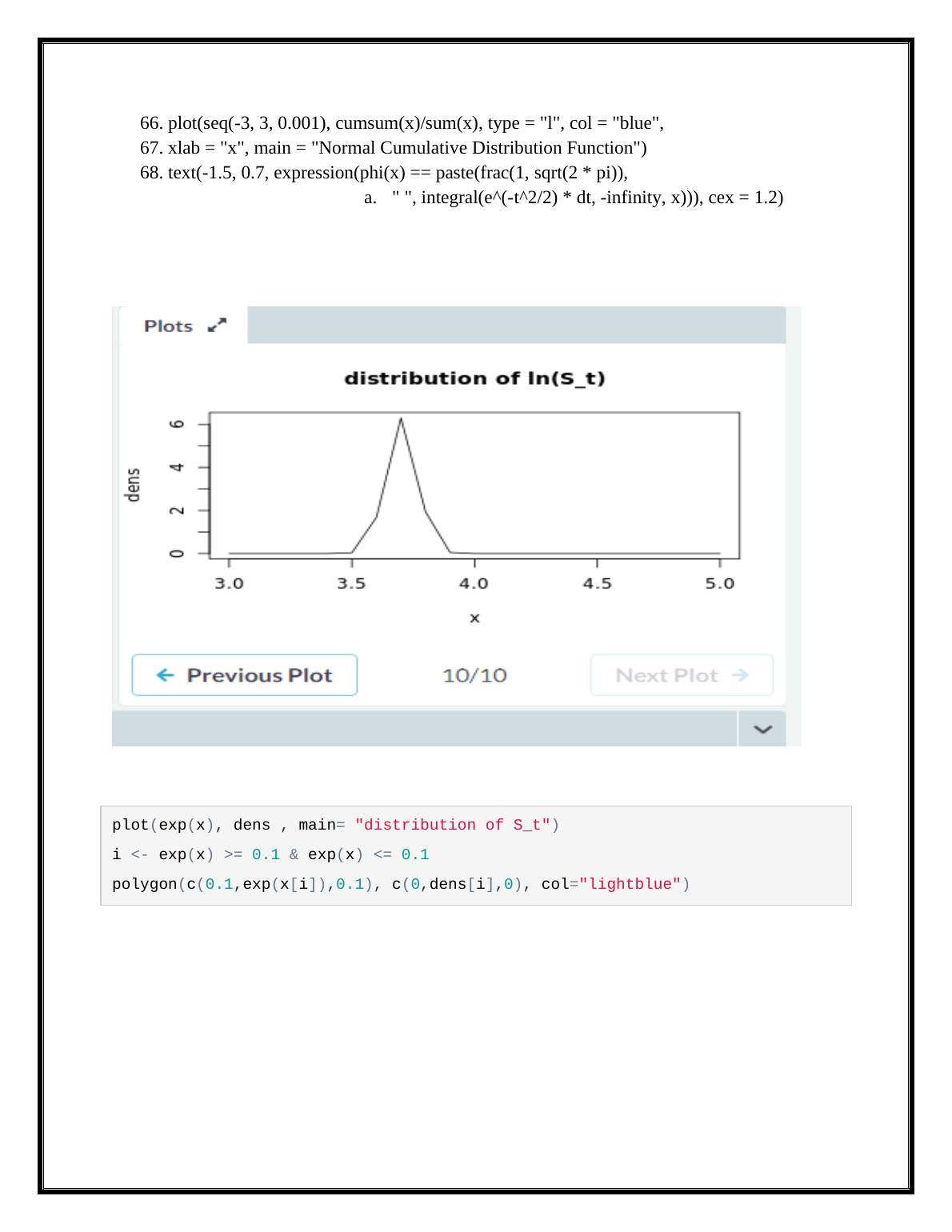
This code simulates stock price and calculates option prices using Black-Scholes model. It also plots the distribution of stock prices and option prices.

1. S0 <- 40
2. mu <- 16/100
3. sd <- 20/100
4. T <- 0.1
5. mean <- log(S0) + (mu-sd^2/2)*T
6. (var <- sd^2*T)
7. (stdev <- sqrt(var))
8. # CI of ln(S_T)
9. CI <- c(mean-0.1*stdev, mean+0.1*stdev)
10. # Plot distribution
11. x <- seq(3,5,by = 0.1)
12. dens <- dnorm(x,mean = mean, sd = stdev)
13. plot(x , dens , main= "distribution of ln(S_t)")
14. i <- x >= 0.1 & x <= 0.1
15. polygon(c(0.1,x[i],0.1), c(0,dens[i],0), col="lightblue")
16. CI2 <- exp(CI)
17. plot(exp(x), dens , main= "distribution of S_t")
18. i <- exp(x) >= 0.1 & exp(x) <= 0.1
19. polygon(c(0.1,exp(x[i]),0.1), c(0,dens[i],0), col="lightblue")
20. (mu <- 0.17 - 0.1^2/2)
21. (sd <- 0.1) # percent
22. # CI for returns =
23. c(mu-0.1*sd, mu+0.1*sd)
24. x <- seq(-0.5,0.8,by = .01)
25. dens <- dnorm(x,mean = mu, sd = sd)
26. plot(x , dens , type='l', main= "distribution of ln(S_t)")
27. i <- x >= -0.1 & x <= 0.1
28. polygon(c(-0.1,x[i],0.1), c(0,dens[i],0), col="lightblue")
29. Call <- function(S, K, r, T, sigma) {
30. d1 <- (log(S/K) + (r + sigma^2/2)*T) / (sigma*sqrt(T))
31. d2 <- d1 - sigma*sqrt(T)
32. S * pnorm(d1) - K*exp(-r*T)*pnorm(d2)
33. }
34. Put <- function(S, K, r, T, sigma) {
35. d1 <- (log(S/K) + (r + sigma^2/2)*T) / (sigma*sqrt(T))
36. d2 <- d1 - sigma*sqrt(T)

37. -S * pnorm(-d1) + K*exp(-r*T)*pnorm(-d2)
38. }
39. # Parameters
40. S <- 100
41. K <- 70
42. T <- 1 # seq(10/52,1/52,-1/52)
43. sigma <- c(.16,.21,.3, .4,.5,.6,.75,1,1.06)
44. d1 <- (log(S/K) + (r + sigma^2/2)*T) / (sigma*sqrt(T))
45. d2 <- d1 - sigma*sqrt(T)
46. p <- cbind(S, K, T, sigma, p = -S * pnorm(-d1) + K*exp(-r*T)*pnorm(-d2))
47. c <- cbind(S, K, T, sigma, c = S * pnorm(d1) - K*exp(-r*T)*pnorm(d2))
48. pnorm(d2) %>% round(2)
49. cprct <- c[,c(1,5)] / matrix(rep(c[1,c(1,5)],each=length(c[,5]) ),ncol = 2) * 100
50. ts.plot(cprct, col = c(1,4), main = "Evolution of Stocks and Calls in %")
51. legend('topleft', c(paste("Stock +", tail(cprct,1)[1]-100, "%") ,
i. paste("Long Call +", round(tail(cprct,1)[2])-100, "%")),
52. col=c(1,4), lty=1)
53. pprct <- p[,c(1,5)] / matrix(rep(p[1,c(1,5)],each=length(c[,5]) ),ncol = 2) * 100
54. ts.plot(pprct, col=1:2, main = "Evolution of Stocks and Puts in %")
55. c[,5] + K*exp(-r*T)
56. p[,5] + S %>% round(1)
57. ## [1] "Implicit Volatility is around 47.5 %)"
58. u <- 0
59. sd <- 0.1
60. x <- rlnorm(10000, mu,sd)
61. plot(density(x), xlim=c(0,1)) ; abline(v=c(1, 1.5), lty=2)
62. par(mfrow = c(1, 1))
63. curve(dnorm, from = -1, to = 3, n = 1000, main = "Normal Probability Density
Function")
64. text(-2, 0.1, expression(f(x) == paste(frac(1, sqrt(2 * pi * sigma^2)),
1. " ", e^{
2. frac(-(x - mu)^2, 2 * sigma^2)
3. })), cex = 1.2)
65. x <- dnorm(seq(-3, 3, 0.001))

66. plot(seq(-3, 3, 0.001), cumsum(x)/sum(x), type = "l", col = "blue",
67. xlab = "x", main = "Normal Cumulative Distribution Function")
68. text(-1.5, 0.7, expression(phi(x) == paste(frac(1, sqrt(2 * pi)),
a. " ", integral(e^(-t^2/2) * dt, -infinity, x))), cex = 1.2)
plot(exp(x), dens , main= "distribution of S_t")
i <- exp(x) >= 0.1 & exp(x) <= 0.1
polygon(c(0.1,exp(x[i]),0.1), c(0,dens[i],0), col="lightblue")