DSP applications and arm technology PDF
VerifiedAdded on 2021/10/08
|25
|4783
|186
AI Summary
Contribute Materials
Your contribution can guide someone’s learning journey. Share your
documents today.
Running head: DSP APPLICATIONS AND ARM TECHNOLOGY
DSP APPLICATIONS AND ARM TECHNOLOGY
Name of the Student
Name of the University
Author Note
DSP APPLICATIONS AND ARM TECHNOLOGY
Name of the Student
Name of the University
Author Note
Secure Best Marks with AI Grader
Need help grading? Try our AI Grader for instant feedback on your assignments.
1DSP APPLICATIONS AND ARM TECHNOLOGY
Table of Contents
Introduction:...............................................................................................................................2
Methodology and obtained results:............................................................................................2
Part 1: Speech Vocoder programmed in MATLAB...............................................................2
MATLAB code for processing the 1st channel:......................................................................3
Part 2: Digital filter bank on ARM STM32F407 Discovery board......................................11
Equivalent C code for signal generation:.............................................................................17
Conclusions:.............................................................................................................................23
References:...............................................................................................................................24
2DSP APPLICATIONS AND ARM TECHNOLOGY
Introduction:
This particular project is divided in two parts. The first part is the implementation of a speech
Vocoder through MATLAB. The Vocoder is basically a software that can synthesize a sound
by speech analysis and then produce the speech in a form which is known as the ‘Shannon
Speech’. Basically at first in the Vocoder the sound is segmented into different channels and
then the sound is rectified by half wave rectifiers. Then it is passed through various low pass
filters and then additive Gaussian white noise is applied to each signal. Then the noise is
filtered through some previously designed filter and finally the output signal is produced by
summing all the filtered signals (Ahammed et al. 2015). This output signal gives clearer
audio than the original signal. Now, the sampling rate that is used in the 3rd order Butterworth
filter is 22.5 KHz as obtained while reading the sound wave in MATLAB. Although the
different kinds of filters can be used to extract the cut off frequencies at 160 Hz, like 3rd and
6th order elliptical filter, Butterworth filter but investigating the different possibilities it is
found that Butterworth produces low pass filtered signals better than any other method
(Sandhu, Kaur and Kaur 2016). Now, the 3rd order elliptical filter is used in the initial
analysis filter of different components of the sound signal (Podder et al. 2014). The filtered
signals are compared based on their frequency spectrum also. Finally, the synthesised and
summed up all the component sound wave is needed to be played with the sound function in
MATLAB to find the difference between the original signal and the synthesized signal.
In the second part a C/C++ code is needed to be designed which acts as a digital filter bank
on the ARM STM32F407 Discovery board. As specified in the question the input signal to
the A/D converter of the digital filter bank of the board is a superimposed three sinusoids of
frequency 500 Hz, 1500 Hz and 2500 Hz respectively. This signal is generated in MATLAB
first and the equivalent code in C is developed by MATLAB Coder. After that, among all the
possibilities of different filters the 10th order Butterworth filter is used for filtering the
individual frequency components as the stop-band Butterworth filter suppresses the stop-band
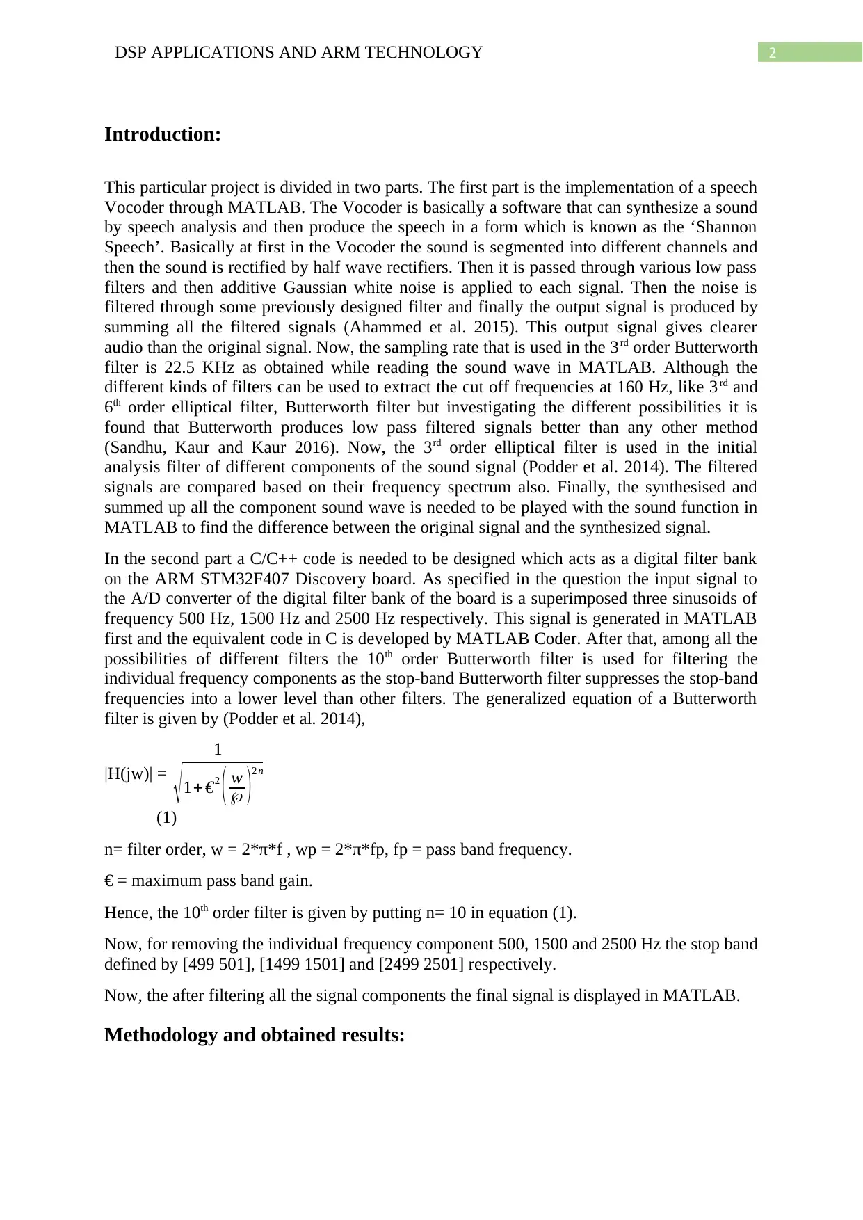
frequencies into a lower level than other filters. The generalized equation of a Butterworth
filter is given by (Podder et al. 2014),
|H(jw)| =
1
√1+€2
( w
℘ )2 n
(1)
n= filter order, w = 2*π*f , wp = 2*π*fp, fp = pass band frequency.
€ = maximum pass band gain.
Hence, the 10th order filter is given by putting n= 10 in equation (1).
Now, for removing the individual frequency component 500, 1500 and 2500 Hz the stop band
defined by [499 501], [1499 1501] and [2499 2501] respectively.
Now, the after filtering all the signal components the final signal is displayed in MATLAB.
Methodology and obtained results:
3DSP APPLICATIONS AND ARM TECHNOLOGY
Part 1: Speech Vocoder programmed in MATLAB
In this part a MATLAB code for Vocoder is needed to be designed and this will be able to
synthesize the sound from the input speech and then produce the ‘Shannon Speech’ (Morise,
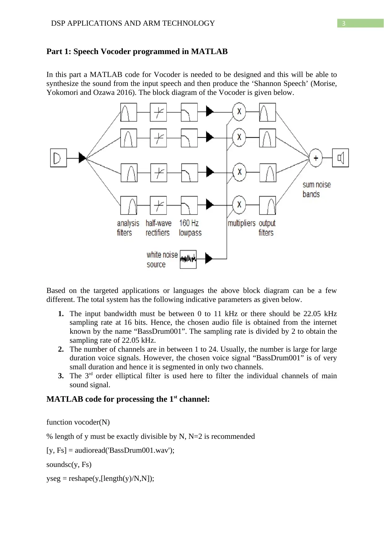
Yokomori and Ozawa 2016). The block diagram of the Vocoder is given below.
Based on the targeted applications or languages the above block diagram can be a few
different. The total system has the following indicative parameters as given below.
1. The input bandwidth must be between 0 to 11 kHz or there should be 22.05 kHz
sampling rate at 16 bits. Hence, the chosen audio file is obtained from the internet
known by the name “BassDrum001”. The sampling rate is divided by 2 to obtain the
sampling rate of 22.05 kHz.
2. The number of channels are in between 1 to 24. Usually, the number is large for large
duration voice signals. However, the chosen voice signal “BassDrum001” is of very
small duration and hence it is segmented in only two channels.
3. The 3rd order elliptical filter is used here to filter the individual channels of main
sound signal.
MATLAB code for processing the 1st channel:
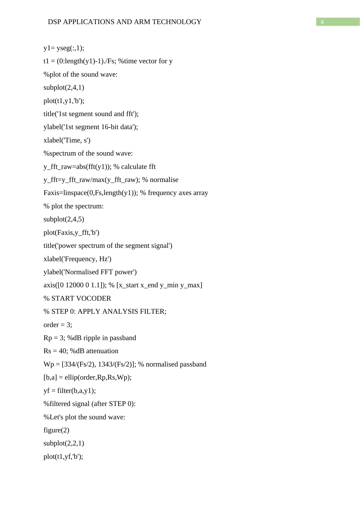
function vocoder(N)
% length of y must be exactly divisible by N, N=2 is recommended
[y, Fs] = audioread('BassDrum001.wav');
soundsc(y, Fs)
yseg = reshape(y,[length(y)/N,N]);
Secure Best Marks with AI Grader
Need help grading? Try our AI Grader for instant feedback on your assignments.
4DSP APPLICATIONS AND ARM TECHNOLOGY
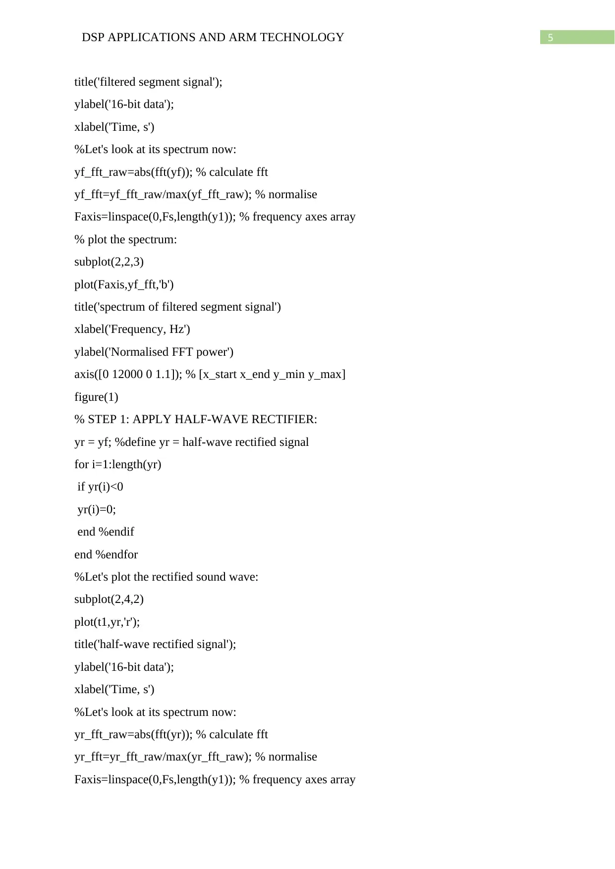
y1= yseg(:,1);
t1 = (0:length(y1)-1)./Fs; %time vector for y
%plot of the sound wave:
subplot(2,4,1)
plot(t1,y1,'b');
title('1st segment sound and fft');
ylabel('1st segment 16-bit data');
xlabel('Time, s')
%spectrum of the sound wave:
y_fft_raw=abs(fft(y1)); % calculate fft
y_fft=y_fft_raw/max(y_fft_raw); % normalise
Faxis=linspace(0,Fs,length(y1)); % frequency axes array
% plot the spectrum:
subplot(2,4,5)
plot(Faxis,y_fft,'b')
title('power spectrum of the segment signal')
xlabel('Frequency, Hz')
ylabel('Normalised FFT power')
axis([0 12000 0 1.1]); % [x_start x_end y_min y_max]
% START VOCODER
% STEP 0: APPLY ANALYSIS FILTER;
order = 3;
Rp = 3; %dB ripple in passband
Rs = 40; %dB attenuation
Wp = [334/(Fs/2), 1343/(Fs/2)]; % normalised passband
[b,a] = ellip(order,Rp,Rs,Wp);
yf = filter(b,a,y1);
%filtered signal (after STEP 0):
%Let's plot the sound wave:
figure(2)
subplot(2,2,1)
plot(t1,yf,'b');
5DSP APPLICATIONS AND ARM TECHNOLOGY
title('filtered segment signal');
ylabel('16-bit data');
xlabel('Time, s')
%Let's look at its spectrum now:
yf_fft_raw=abs(fft(yf)); % calculate fft
yf_fft=yf_fft_raw/max(yf_fft_raw); % normalise
Faxis=linspace(0,Fs,length(y1)); % frequency axes array
% plot the spectrum:
subplot(2,2,3)
plot(Faxis,yf_fft,'b')
title('spectrum of filtered segment signal')
xlabel('Frequency, Hz')
ylabel('Normalised FFT power')
axis([0 12000 0 1.1]); % [x_start x_end y_min y_max]
figure(1)
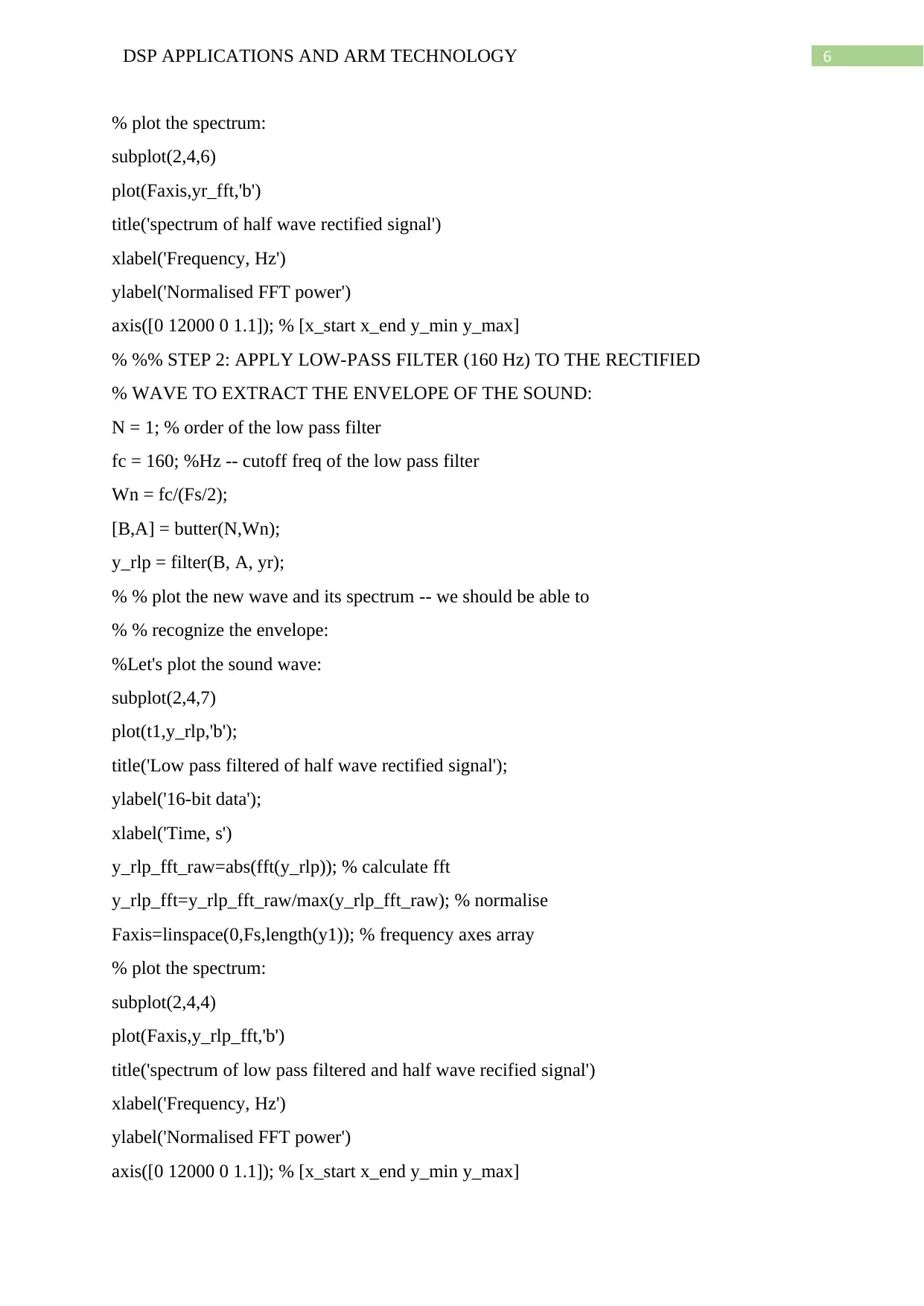
% STEP 1: APPLY HALF-WAVE RECTIFIER:
yr = yf; %define yr = half-wave rectified signal
for i=1:length(yr)
if yr(i)<0
yr(i)=0;
end %endif
end %endfor
%Let's plot the rectified sound wave:
subplot(2,4,2)
plot(t1,yr,'r');
title('half-wave rectified signal');
ylabel('16-bit data');
xlabel('Time, s')
%Let's look at its spectrum now:
yr_fft_raw=abs(fft(yr)); % calculate fft
yr_fft=yr_fft_raw/max(yr_fft_raw); % normalise
Faxis=linspace(0,Fs,length(y1)); % frequency axes array
6DSP APPLICATIONS AND ARM TECHNOLOGY
% plot the spectrum:
subplot(2,4,6)
plot(Faxis,yr_fft,'b')
title('spectrum of half wave rectified signal')
xlabel('Frequency, Hz')
ylabel('Normalised FFT power')
axis([0 12000 0 1.1]); % [x_start x_end y_min y_max]
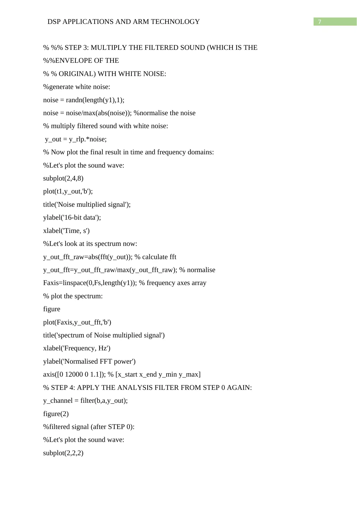
% %% STEP 2: APPLY LOW-PASS FILTER (160 Hz) TO THE RECTIFIED
% WAVE TO EXTRACT THE ENVELOPE OF THE SOUND:
N = 1; % order of the low pass filter
fc = 160; %Hz -- cutoff freq of the low pass filter
Wn = fc/(Fs/2);
[B,A] = butter(N,Wn);
y_rlp = filter(B, A, yr);
% % plot the new wave and its spectrum -- we should be able to
% % recognize the envelope:
%Let's plot the sound wave:
subplot(2,4,7)
plot(t1,y_rlp,'b');
title('Low pass filtered of half wave rectified signal');
ylabel('16-bit data');
xlabel('Time, s')
y_rlp_fft_raw=abs(fft(y_rlp)); % calculate fft
y_rlp_fft=y_rlp_fft_raw/max(y_rlp_fft_raw); % normalise
Faxis=linspace(0,Fs,length(y1)); % frequency axes array
% plot the spectrum:
subplot(2,4,4)
plot(Faxis,y_rlp_fft,'b')
title('spectrum of low pass filtered and half wave recified signal')
xlabel('Frequency, Hz')
ylabel('Normalised FFT power')
axis([0 12000 0 1.1]); % [x_start x_end y_min y_max]
% plot the spectrum:
subplot(2,4,6)
plot(Faxis,yr_fft,'b')
title('spectrum of half wave rectified signal')
xlabel('Frequency, Hz')
ylabel('Normalised FFT power')
axis([0 12000 0 1.1]); % [x_start x_end y_min y_max]
% %% STEP 2: APPLY LOW-PASS FILTER (160 Hz) TO THE RECTIFIED
% WAVE TO EXTRACT THE ENVELOPE OF THE SOUND:
N = 1; % order of the low pass filter
fc = 160; %Hz -- cutoff freq of the low pass filter
Wn = fc/(Fs/2);
[B,A] = butter(N,Wn);
y_rlp = filter(B, A, yr);
% % plot the new wave and its spectrum -- we should be able to
% % recognize the envelope:
%Let's plot the sound wave:
subplot(2,4,7)
plot(t1,y_rlp,'b');
title('Low pass filtered of half wave rectified signal');
ylabel('16-bit data');
xlabel('Time, s')
y_rlp_fft_raw=abs(fft(y_rlp)); % calculate fft
y_rlp_fft=y_rlp_fft_raw/max(y_rlp_fft_raw); % normalise
Faxis=linspace(0,Fs,length(y1)); % frequency axes array
% plot the spectrum:
subplot(2,4,4)
plot(Faxis,y_rlp_fft,'b')
title('spectrum of low pass filtered and half wave recified signal')
xlabel('Frequency, Hz')
ylabel('Normalised FFT power')
axis([0 12000 0 1.1]); % [x_start x_end y_min y_max]
Paraphrase This Document
Need a fresh take? Get an instant paraphrase of this document with our AI Paraphraser
7DSP APPLICATIONS AND ARM TECHNOLOGY
% %% STEP 3: MULTIPLY THE FILTERED SOUND (WHICH IS THE
%%ENVELOPE OF THE
% % ORIGINAL) WITH WHITE NOISE:
%generate white noise:
noise = randn(length(y1),1);
noise = noise/max(abs(noise)); %normalise the noise
% multiply filtered sound with white noise:
y_out = y_rlp.*noise;
% Now plot the final result in time and frequency domains:
%Let's plot the sound wave:
subplot(2,4,8)
plot(t1,y_out,'b');
title('Noise multiplied signal');
ylabel('16-bit data');
xlabel('Time, s')
%Let's look at its spectrum now:
y_out_fft_raw=abs(fft(y_out)); % calculate fft
y_out_fft=y_out_fft_raw/max(y_out_fft_raw); % normalise
Faxis=linspace(0,Fs,length(y1)); % frequency axes array
% plot the spectrum:
figure
plot(Faxis,y_out_fft,'b')
title('spectrum of Noise multiplied signal')
xlabel('Frequency, Hz')
ylabel('Normalised FFT power')
axis([0 12000 0 1.1]); % [x_start x_end y_min y_max]
% STEP 4: APPLY THE ANALYSIS FILTER FROM STEP 0 AGAIN:
y_channel = filter(b,a,y_out);
figure(2)
%filtered signal (after STEP 0):
%Let's plot the sound wave:
subplot(2,2,2)
8DSP APPLICATIONS AND ARM TECHNOLOGY
plot(t1,y_channel,'b');
title('Noise filtered signal');
ylabel('16-bit data');
xlabel('Time, s')
%Let's look at its spectrum now:
yc_fft_raw=abs(fft(y_channel)); % calculate fft
yc_fft=yc_fft_raw/max(yc_fft_raw); % normalise
Faxis=linspace(0,Fs,length(y_channel)); % frequency axes array
% plot the spectrum:
subplot(2,2,4)
plot(Faxis,yc_fft,'b')
title('Spectrum of Noise filtered signal')
xlabel('Frequency, Hz')
ylabel('Normalised FFT power')
axis([0 12000 0 1.1]); % [x_start x_end y_min y_max]
% % play the vocoded sound
soundsc(y_channel, Fs)
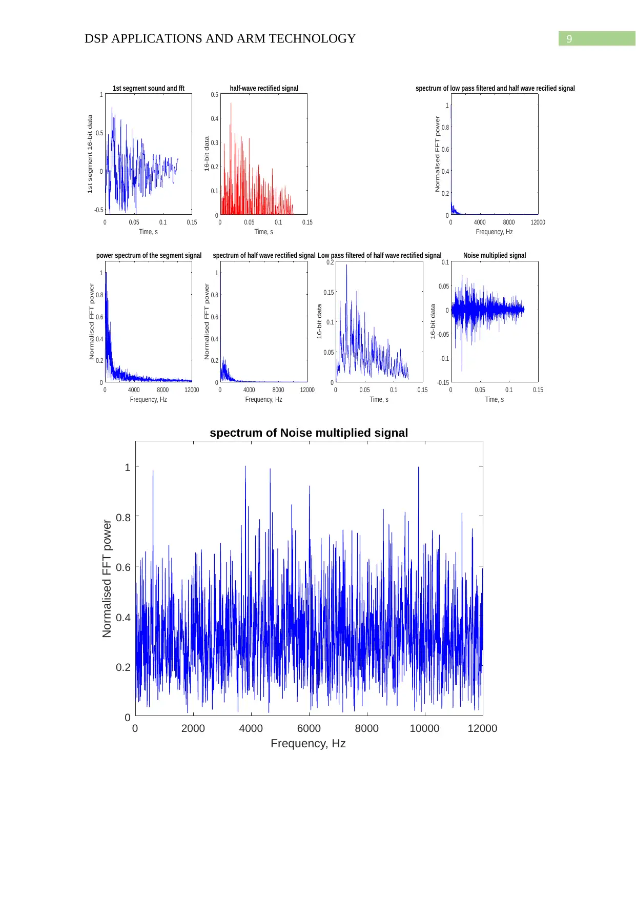
Plots for the 1st segment:
9DSP APPLICATIONS AND ARM TECHNOLOGY
0 0.05 0.1 0.15
Time, s
-0.5
0
0.5
1
1st segment 16-bit data
1st segment sound and fft
0 4000 8000 12000
Frequency, Hz
0
0.2
0.4
0.6
0.8
1
Normalised FFT power
power spectrum of the segment signal
0 0.05 0.1 0.15
Time, s
0
0.1
0.2
0.3
0.4
0.5
16-bit data
half-wave rectified signal
0 4000 8000 12000
Frequency, Hz
0
0.2
0.4
0.6
0.8
1
Normalised FFT power
spectrum of half wave rectified signal
0 0.05 0.1 0.15
Time, s
0
0.05
0.1
0.15
0.2
16-bit data
Low pass filtered of half wave rectified signal
0 4000 8000 12000
Frequency, Hz
0
0.2
0.4
0.6
0.8
1
Normalised FFT power
spectrum of low pass filtered and half wave recified signal
0 0.05 0.1 0.15
Time, s
-0.15
-0.1
-0.05
0
0.05
0.1
16-bit data
Noise multiplied signal
0 2000 4000 6000 8000 10000 12000
Frequency, Hz
0
0.2
0.4
0.6
0.8
1
Normalised FFT power
spectrum of Noise multiplied signal
0 0.05 0.1 0.15
Time, s
-0.5
0
0.5
1
1st segment 16-bit data
1st segment sound and fft
0 4000 8000 12000
Frequency, Hz
0
0.2
0.4
0.6
0.8
1
Normalised FFT power
power spectrum of the segment signal
0 0.05 0.1 0.15
Time, s
0
0.1
0.2
0.3
0.4
0.5
16-bit data
half-wave rectified signal
0 4000 8000 12000
Frequency, Hz
0
0.2
0.4
0.6
0.8
1
Normalised FFT power
spectrum of half wave rectified signal
0 0.05 0.1 0.15
Time, s
0
0.05
0.1
0.15
0.2
16-bit data
Low pass filtered of half wave rectified signal
0 4000 8000 12000
Frequency, Hz
0
0.2
0.4
0.6
0.8
1
Normalised FFT power
spectrum of low pass filtered and half wave recified signal
0 0.05 0.1 0.15
Time, s
-0.15
-0.1
-0.05
0
0.05
0.1
16-bit data
Noise multiplied signal
0 2000 4000 6000 8000 10000 12000
Frequency, Hz
0
0.2
0.4
0.6
0.8
1
Normalised FFT power
spectrum of Noise multiplied signal
Secure Best Marks with AI Grader
Need help grading? Try our AI Grader for instant feedback on your assignments.
10DSP APPLICATIONS AND ARM TECHNOLOGY
0 0.02 0.04 0.06 0.08 0.1 0.12 0.14
Time, s
-0.5
0
0.5
16-bit data
filtered segment signal
0 2000 4000 6000 8000 10000 12000
Frequency, Hz
0
0.2
0.4
0.6
0.8
1
Normalised FFT power
spectrum of filtered segment signal
0 0.02 0.04 0.06 0.08 0.1 0.12 0.14
Time, s
-0.015
-0.01
-0.005
0
0.005
0.01
0.015
16-bit data
Noise filtered signal
0 2000 4000 6000 8000 10000 12000
Frequency, Hz
0
0.2
0.4
0.6
0.8
1
Normalised FFT power
Spectrum of Noise filtered signal
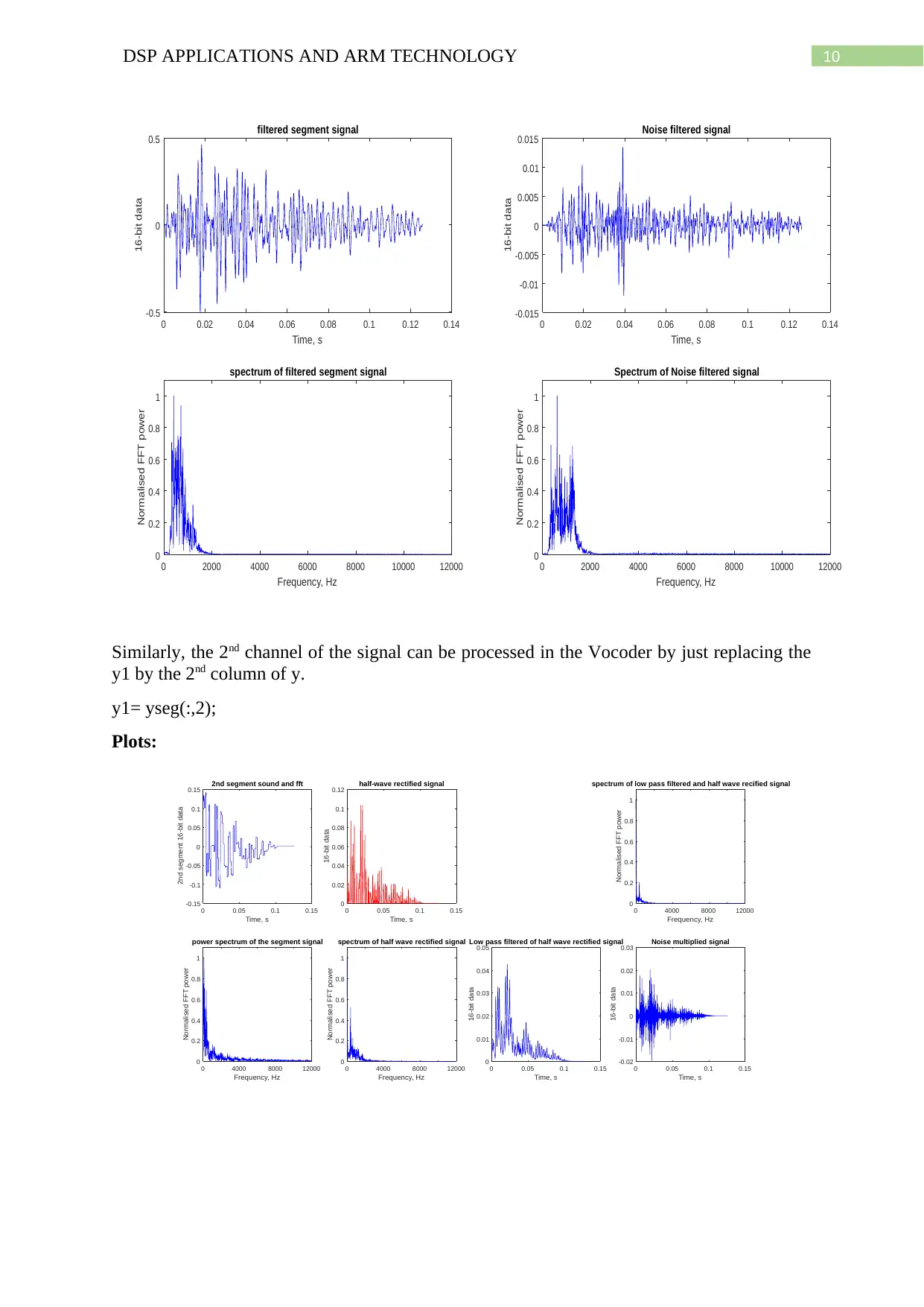
Similarly, the 2nd channel of the signal can be processed in the Vocoder by just replacing the
y1 by the 2nd column of y.
y1= yseg(:,2);
Plots:
0 0.05 0.1 0.15
Time, s
-0.15
-0.1
-0.05
0
0.05
0.1
0.15
2nd segment 16-bit data
2nd segment sound and fft
0 4000 8000 12000
Frequency, Hz
0
0.2
0.4
0.6
0.8
1
Normalised FFT power
power spectrum of the segment signal
0 0.05 0.1 0.15
Time, s
0
0.02
0.04
0.06
0.08
0.1
0.12
16-bit data
half-wave rectified signal
0 4000 8000 12000
Frequency, Hz
0
0.2
0.4
0.6
0.8
1
Normalised FFT power
spectrum of half wave rectified signal
0 0.05 0.1 0.15
Time, s
0
0.01
0.02
0.03
0.04
0.05
16-bit data
Low pass filtered of half wave rectified signal
0 4000 8000 12000
Frequency, Hz
0
0.2
0.4
0.6
0.8
1
Normalised FFT power
spectrum of low pass filtered and half wave recified signal
0 0.05 0.1 0.15
Time, s
-0.02
-0.01
0
0.01
0.02
0.03
16-bit data
Noise multiplied signal
0 0.02 0.04 0.06 0.08 0.1 0.12 0.14
Time, s
-0.5
0
0.5
16-bit data
filtered segment signal
0 2000 4000 6000 8000 10000 12000
Frequency, Hz
0
0.2
0.4
0.6
0.8
1
Normalised FFT power
spectrum of filtered segment signal
0 0.02 0.04 0.06 0.08 0.1 0.12 0.14
Time, s
-0.015
-0.01
-0.005
0
0.005
0.01
0.015
16-bit data
Noise filtered signal
0 2000 4000 6000 8000 10000 12000
Frequency, Hz
0
0.2
0.4
0.6
0.8
1
Normalised FFT power
Spectrum of Noise filtered signal
Similarly, the 2nd channel of the signal can be processed in the Vocoder by just replacing the
y1 by the 2nd column of y.
y1= yseg(:,2);
Plots:
0 0.05 0.1 0.15
Time, s
-0.15
-0.1
-0.05
0
0.05
0.1
0.15
2nd segment 16-bit data
2nd segment sound and fft
0 4000 8000 12000
Frequency, Hz
0
0.2
0.4
0.6
0.8
1
Normalised FFT power
power spectrum of the segment signal
0 0.05 0.1 0.15
Time, s
0
0.02
0.04
0.06
0.08
0.1
0.12
16-bit data
half-wave rectified signal
0 4000 8000 12000
Frequency, Hz
0
0.2
0.4
0.6
0.8
1
Normalised FFT power
spectrum of half wave rectified signal
0 0.05 0.1 0.15
Time, s
0
0.01
0.02
0.03
0.04
0.05
16-bit data
Low pass filtered of half wave rectified signal
0 4000 8000 12000
Frequency, Hz
0
0.2
0.4
0.6
0.8
1
Normalised FFT power
spectrum of low pass filtered and half wave recified signal
0 0.05 0.1 0.15
Time, s
-0.02
-0.01
0
0.01
0.02
0.03
16-bit data
Noise multiplied signal
11DSP APPLICATIONS AND ARM TECHNOLOGY
0 0.02 0.04 0.06 0.08 0.1 0.12 0.14
Time, s
-0.15
-0.1
-0.05
0
0.05
0.1
0.15
16-bit data
filtered segment signal
0 2000 4000 6000 8000 10000 12000
Frequency, Hz
0
0.2
0.4
0.6
0.8
1
Normalised FFT power
spectrum of filtered segment signal
0 0.02 0.04 0.06 0.08 0.1 0.12 0.14
Time, s
-3
-2
-1
0
1
2
16-bit data
10-3 Noise filtered signal
0 2000 4000 6000 8000 10000 12000
Frequency, Hz
0
0.2
0.4
0.6
0.8
1
Normalised FFT power
Spectrum of Noise filtered signal
0 2000 4000 6000 8000 10000 12000
Frequency, Hz
0
0.2
0.4
0.6
0.8
1
Normalised FFT power
spectrum of Noise multiplied signal
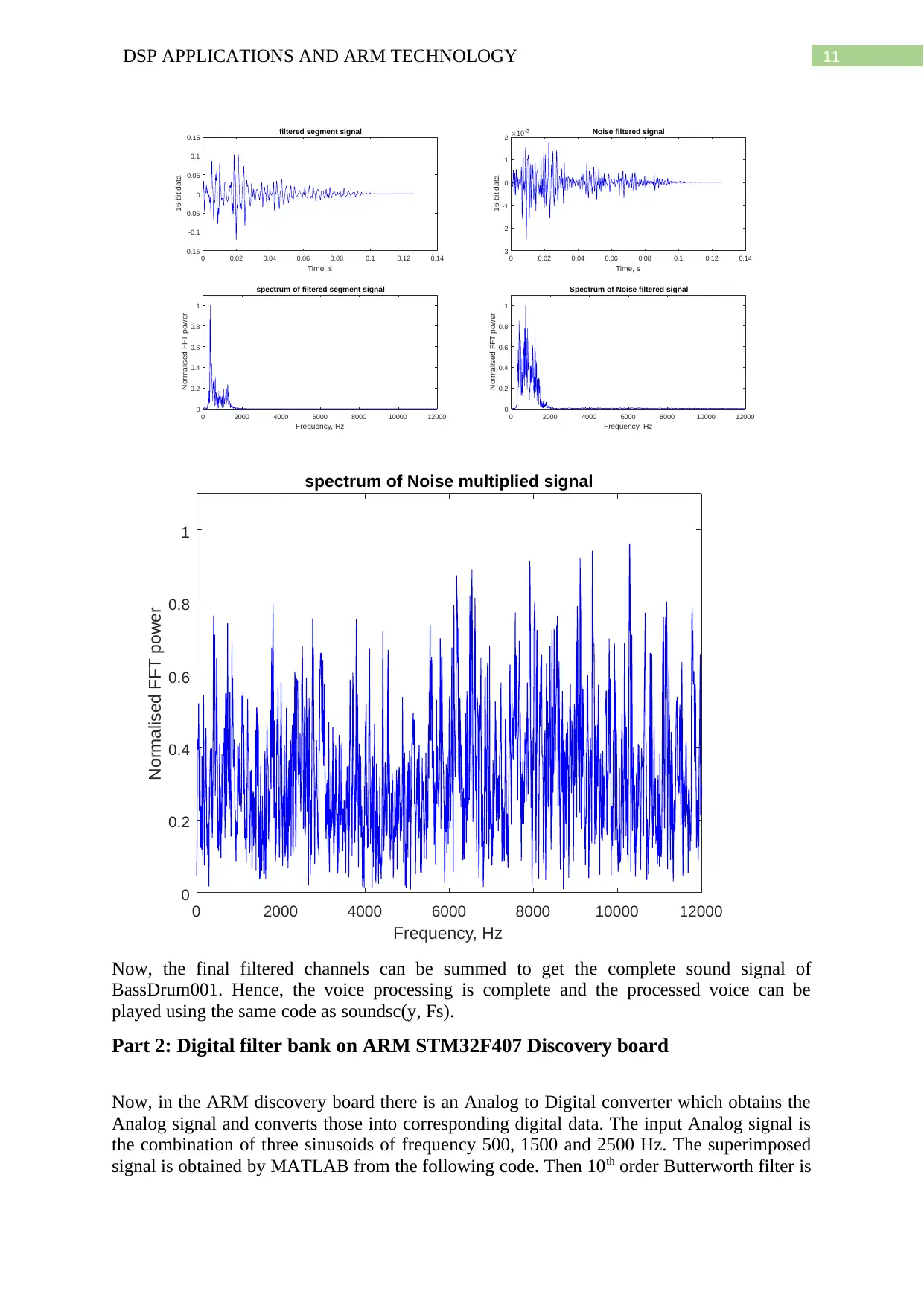
Now, the final filtered channels can be summed to get the complete sound signal of
BassDrum001. Hence, the voice processing is complete and the processed voice can be
played using the same code as soundsc(y, Fs).
Part 2: Digital filter bank on ARM STM32F407 Discovery board
Now, in the ARM discovery board there is an Analog to Digital converter which obtains the
Analog signal and converts those into corresponding digital data. The input Analog signal is
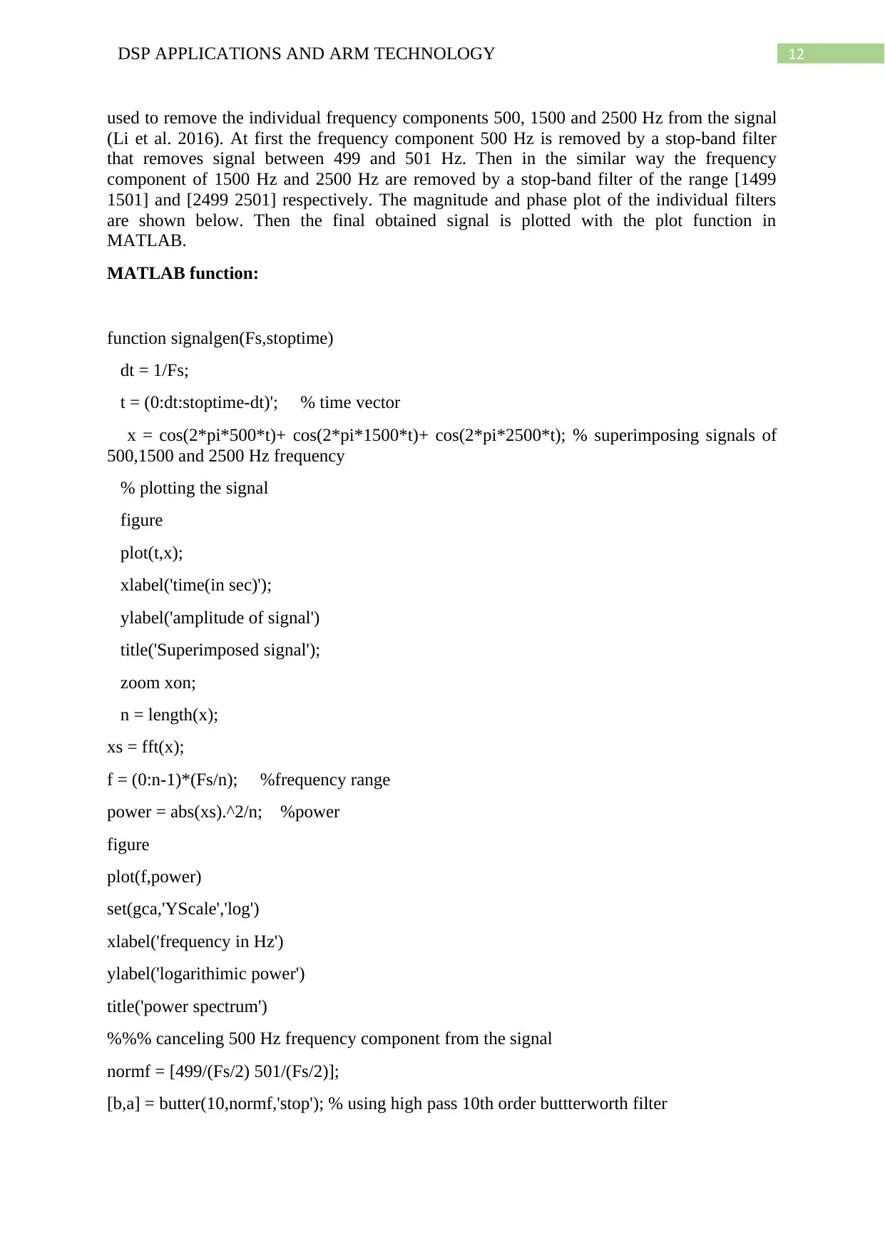
the combination of three sinusoids of frequency 500, 1500 and 2500 Hz. The superimposed
signal is obtained by MATLAB from the following code. Then 10th order Butterworth filter is
0 0.02 0.04 0.06 0.08 0.1 0.12 0.14
Time, s
-0.15
-0.1
-0.05
0
0.05
0.1
0.15
16-bit data
filtered segment signal
0 2000 4000 6000 8000 10000 12000
Frequency, Hz
0
0.2
0.4
0.6
0.8
1
Normalised FFT power
spectrum of filtered segment signal
0 0.02 0.04 0.06 0.08 0.1 0.12 0.14
Time, s
-3
-2
-1
0
1
2
16-bit data
10-3 Noise filtered signal
0 2000 4000 6000 8000 10000 12000
Frequency, Hz
0
0.2
0.4
0.6
0.8
1
Normalised FFT power
Spectrum of Noise filtered signal
0 2000 4000 6000 8000 10000 12000
Frequency, Hz
0
0.2
0.4
0.6
0.8
1
Normalised FFT power
spectrum of Noise multiplied signal
Now, the final filtered channels can be summed to get the complete sound signal of
BassDrum001. Hence, the voice processing is complete and the processed voice can be
played using the same code as soundsc(y, Fs).
Part 2: Digital filter bank on ARM STM32F407 Discovery board
Now, in the ARM discovery board there is an Analog to Digital converter which obtains the
Analog signal and converts those into corresponding digital data. The input Analog signal is
the combination of three sinusoids of frequency 500, 1500 and 2500 Hz. The superimposed
signal is obtained by MATLAB from the following code. Then 10th order Butterworth filter is
12DSP APPLICATIONS AND ARM TECHNOLOGY
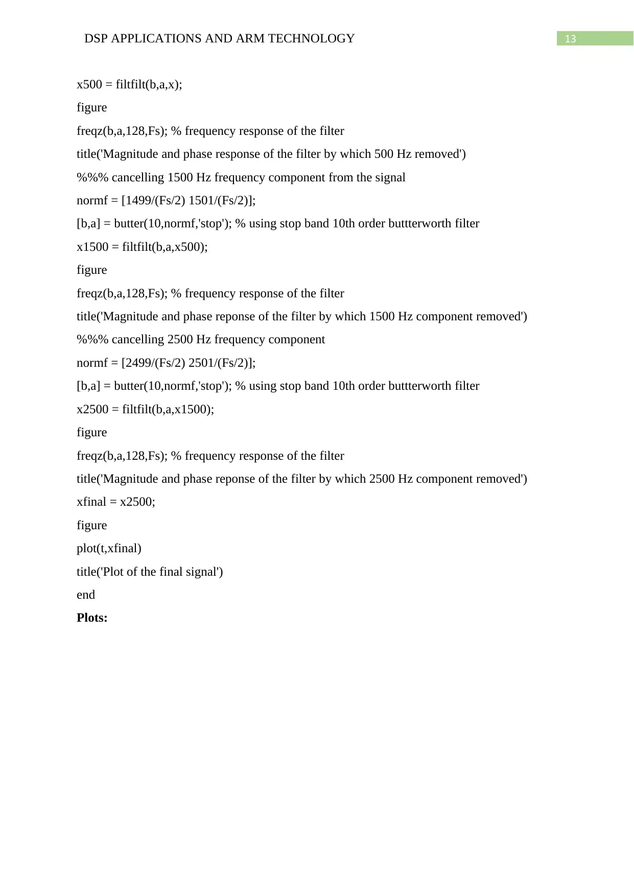
used to remove the individual frequency components 500, 1500 and 2500 Hz from the signal
(Li et al. 2016). At first the frequency component 500 Hz is removed by a stop-band filter
that removes signal between 499 and 501 Hz. Then in the similar way the frequency
component of 1500 Hz and 2500 Hz are removed by a stop-band filter of the range [1499
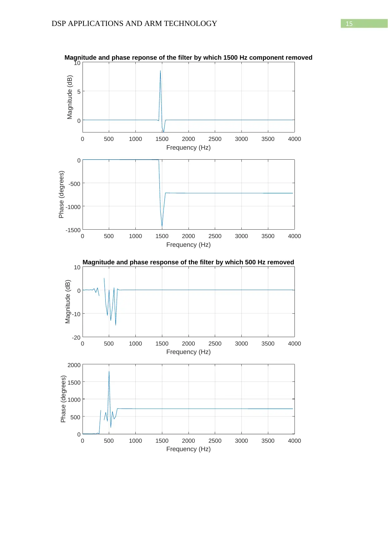
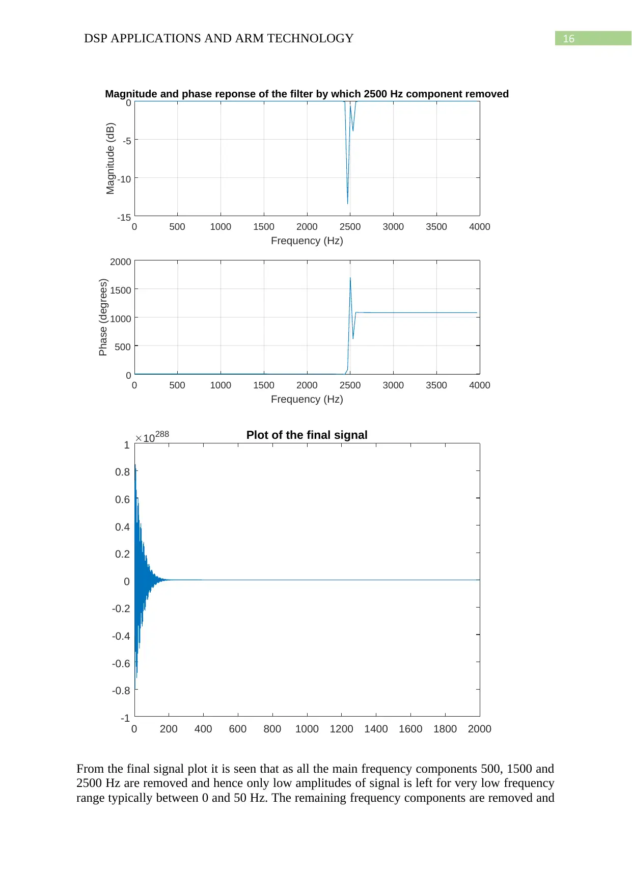
1501] and [2499 2501] respectively. The magnitude and phase plot of the individual filters
are shown below. Then the final obtained signal is plotted with the plot function in
MATLAB.
MATLAB function:
function signalgen(Fs,stoptime)
dt = 1/Fs;
t = (0:dt:stoptime-dt)'; % time vector
x = cos(2*pi*500*t)+ cos(2*pi*1500*t)+ cos(2*pi*2500*t); % superimposing signals of
500,1500 and 2500 Hz frequency
% plotting the signal
figure
plot(t,x);
xlabel('time(in sec)');
ylabel('amplitude of signal')
title('Superimposed signal');
zoom xon;
n = length(x);
xs = fft(x);
f = (0:n-1)*(Fs/n); %frequency range
power = abs(xs).^2/n; %power
figure
plot(f,power)
set(gca,'YScale','log')
xlabel('frequency in Hz')
ylabel('logarithimic power')
title('power spectrum')
%%% canceling 500 Hz frequency component from the signal
normf = [499/(Fs/2) 501/(Fs/2)];
[b,a] = butter(10,normf,'stop'); % using high pass 10th order buttterworth filter
Paraphrase This Document
Need a fresh take? Get an instant paraphrase of this document with our AI Paraphraser
13DSP APPLICATIONS AND ARM TECHNOLOGY
x500 = filtfilt(b,a,x);
figure
freqz(b,a,128,Fs); % frequency response of the filter
title('Magnitude and phase response of the filter by which 500 Hz removed')
%%% cancelling 1500 Hz frequency component from the signal
normf = [1499/(Fs/2) 1501/(Fs/2)];
[b,a] = butter(10,normf,'stop'); % using stop band 10th order buttterworth filter
x1500 = filtfilt(b,a,x500);
figure
freqz(b,a,128,Fs); % frequency response of the filter
title('Magnitude and phase reponse of the filter by which 1500 Hz component removed')
%%% cancelling 2500 Hz frequency component
normf = [2499/(Fs/2) 2501/(Fs/2)];
[b,a] = butter(10,normf,'stop'); % using stop band 10th order buttterworth filter
x2500 = filtfilt(b,a,x1500);
figure
freqz(b,a,128,Fs); % frequency response of the filter
title('Magnitude and phase reponse of the filter by which 2500 Hz component removed')
xfinal = x2500;
figure
plot(t,xfinal)
title('Plot of the final signal')
end
Plots:
14DSP APPLICATIONS AND ARM TECHNOLOGY
0 0.05 0.1 0.15 0.2 0.25
time(in sec)
-3
-2
-1
0
1
2
3
amplitude of signal
Superimposed signal
0 1000 2000 3000 4000 5000 6000 7000 8000
frequency in Hz
10 -30
10 -25
10 -20
10 -15
10 -10
10 -5
10 0
10 5
logarithimic power
power spectrum
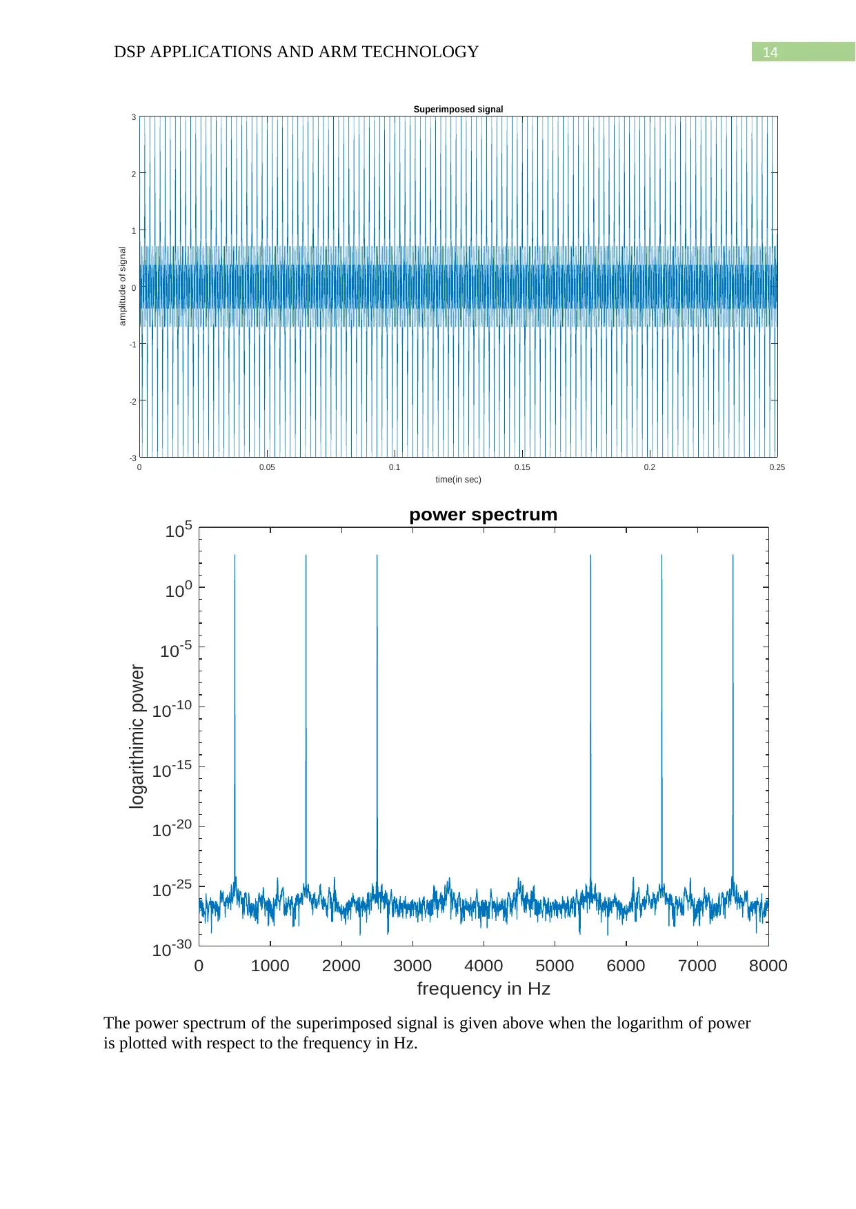
The power spectrum of the superimposed signal is given above when the logarithm of power
is plotted with respect to the frequency in Hz.
15DSP APPLICATIONS AND ARM TECHNOLOGY
0 500 1000 1500 2000 2500 3000 3500 4000
Frequency (Hz)
-1500
-1000
-500
0
Phase (degrees)
0 500 1000 1500 2000 2500 3000 3500 4000
Frequency (Hz)
0
5
10
Magnitude (dB)
Magnitude and phase reponse of the filter by which 1500 Hz component removed
0 500 1000 1500 2000 2500 3000 3500 4000
Frequency (Hz)
0
500
1000
1500
2000
Phase (degrees)
0 500 1000 1500 2000 2500 3000 3500 4000
Frequency (Hz)
-20
-10
0
10
Magnitude (dB)
Magnitude and phase response of the filter by which 500 Hz removed
0 500 1000 1500 2000 2500 3000 3500 4000
Frequency (Hz)
-1500
-1000
-500
0
Phase (degrees)
0 500 1000 1500 2000 2500 3000 3500 4000
Frequency (Hz)
0
5
10
Magnitude (dB)
Magnitude and phase reponse of the filter by which 1500 Hz component removed
0 500 1000 1500 2000 2500 3000 3500 4000
Frequency (Hz)
0
500
1000
1500
2000
Phase (degrees)
0 500 1000 1500 2000 2500 3000 3500 4000
Frequency (Hz)
-20
-10
0
10
Magnitude (dB)
Magnitude and phase response of the filter by which 500 Hz removed
Secure Best Marks with AI Grader
Need help grading? Try our AI Grader for instant feedback on your assignments.
16DSP APPLICATIONS AND ARM TECHNOLOGY
0 500 1000 1500 2000 2500 3000 3500 4000
Frequency (Hz)
0
500
1000
1500
2000
Phase (degrees)
0 500 1000 1500 2000 2500 3000 3500 4000
Frequency (Hz)
-15
-10
-5
0
Magnitude (dB)
Magnitude and phase reponse of the filter by which 2500 Hz component removed
0 200 400 600 800 1000 1200 1400 1600 1800 2000
-1
-0.8
-0.6
-0.4
-0.2
0
0.2
0.4
0.6
0.8
1 10288 Plot of the final signal
From the final signal plot it is seen that as all the main frequency components 500, 1500 and
2500 Hz are removed and hence only low amplitudes of signal is left for very low frequency
range typically between 0 and 50 Hz. The remaining frequency components are removed and
0 500 1000 1500 2000 2500 3000 3500 4000
Frequency (Hz)
0
500
1000
1500
2000
Phase (degrees)
0 500 1000 1500 2000 2500 3000 3500 4000
Frequency (Hz)
-15
-10
-5
0
Magnitude (dB)
Magnitude and phase reponse of the filter by which 2500 Hz component removed
0 200 400 600 800 1000 1200 1400 1600 1800 2000
-1
-0.8
-0.6
-0.4
-0.2
0
0.2
0.4
0.6
0.8
1 10288 Plot of the final signal
From the final signal plot it is seen that as all the main frequency components 500, 1500 and
2500 Hz are removed and hence only low amplitudes of signal is left for very low frequency
range typically between 0 and 50 Hz. The remaining frequency components are removed and
17DSP APPLICATIONS AND ARM TECHNOLOGY
hence it is seen that the amplitude goes to zero for higher frequency components. Now, the
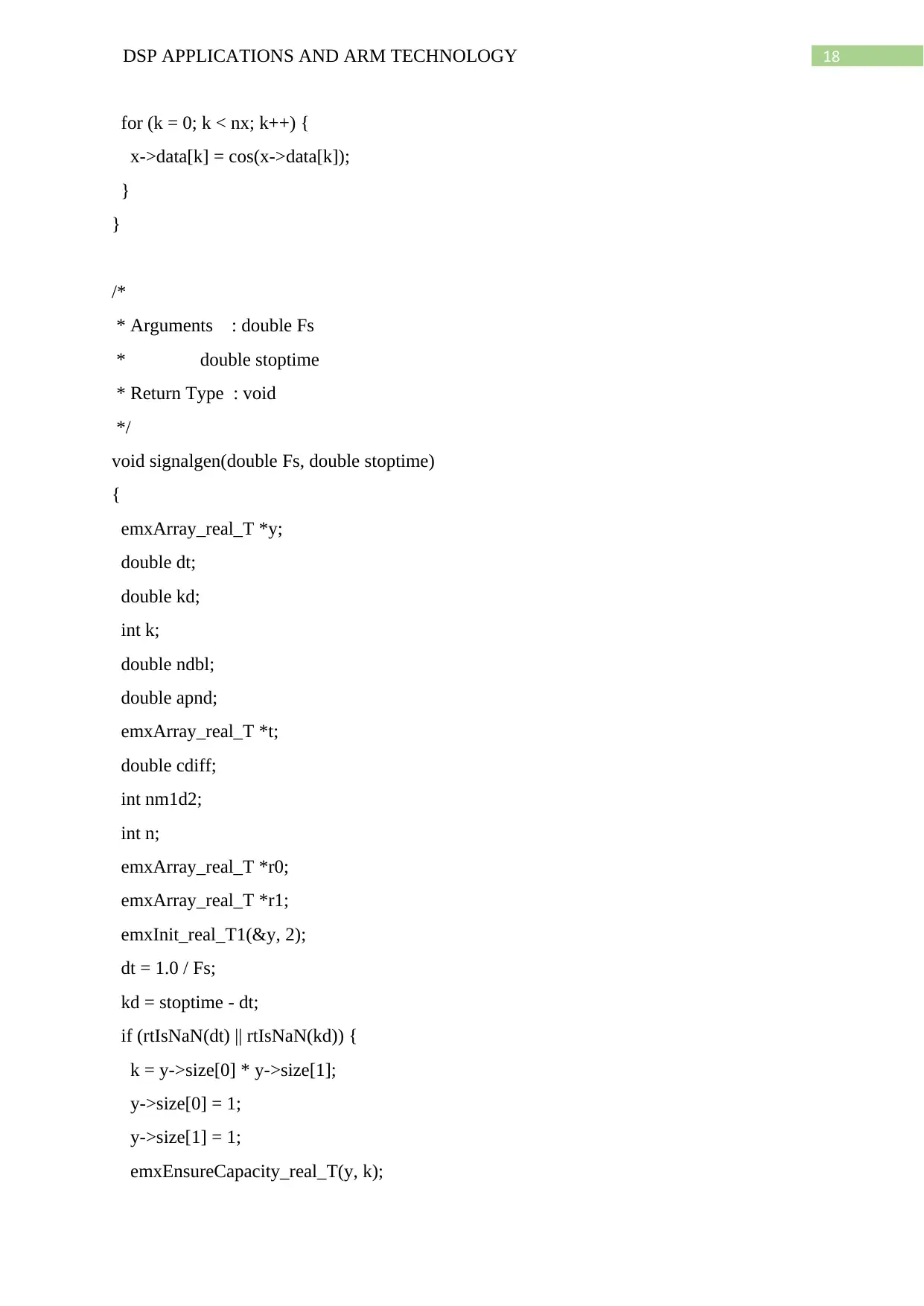
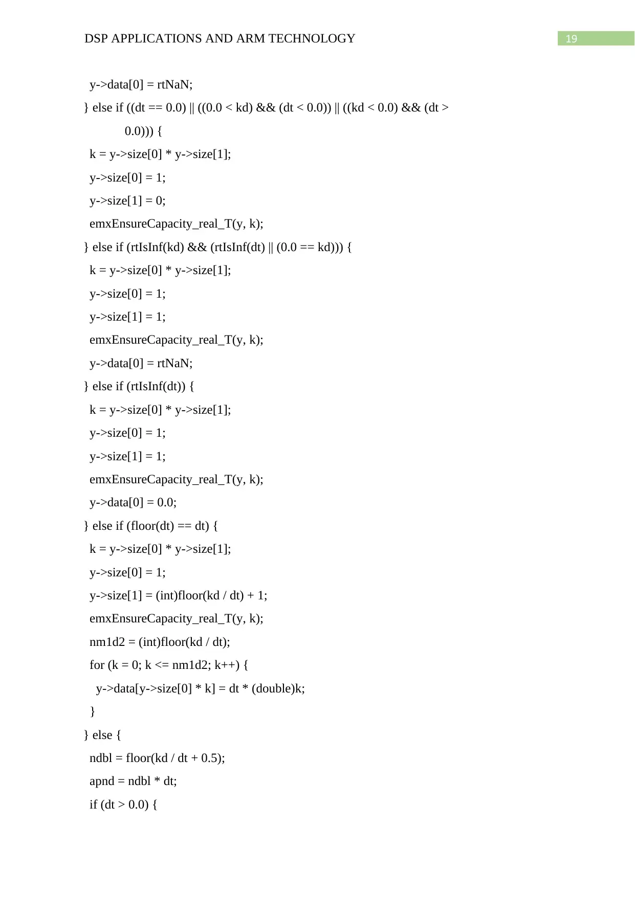
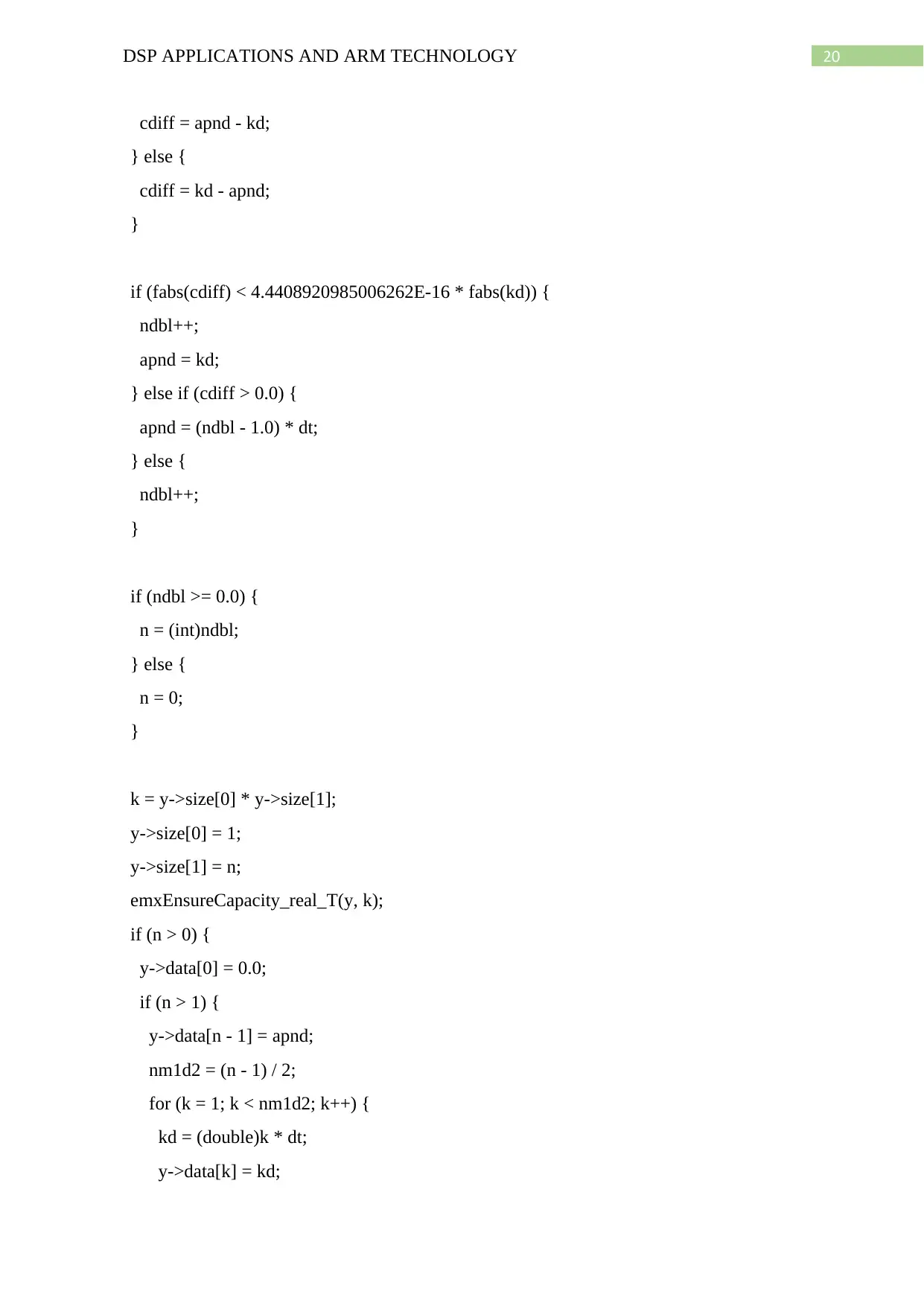
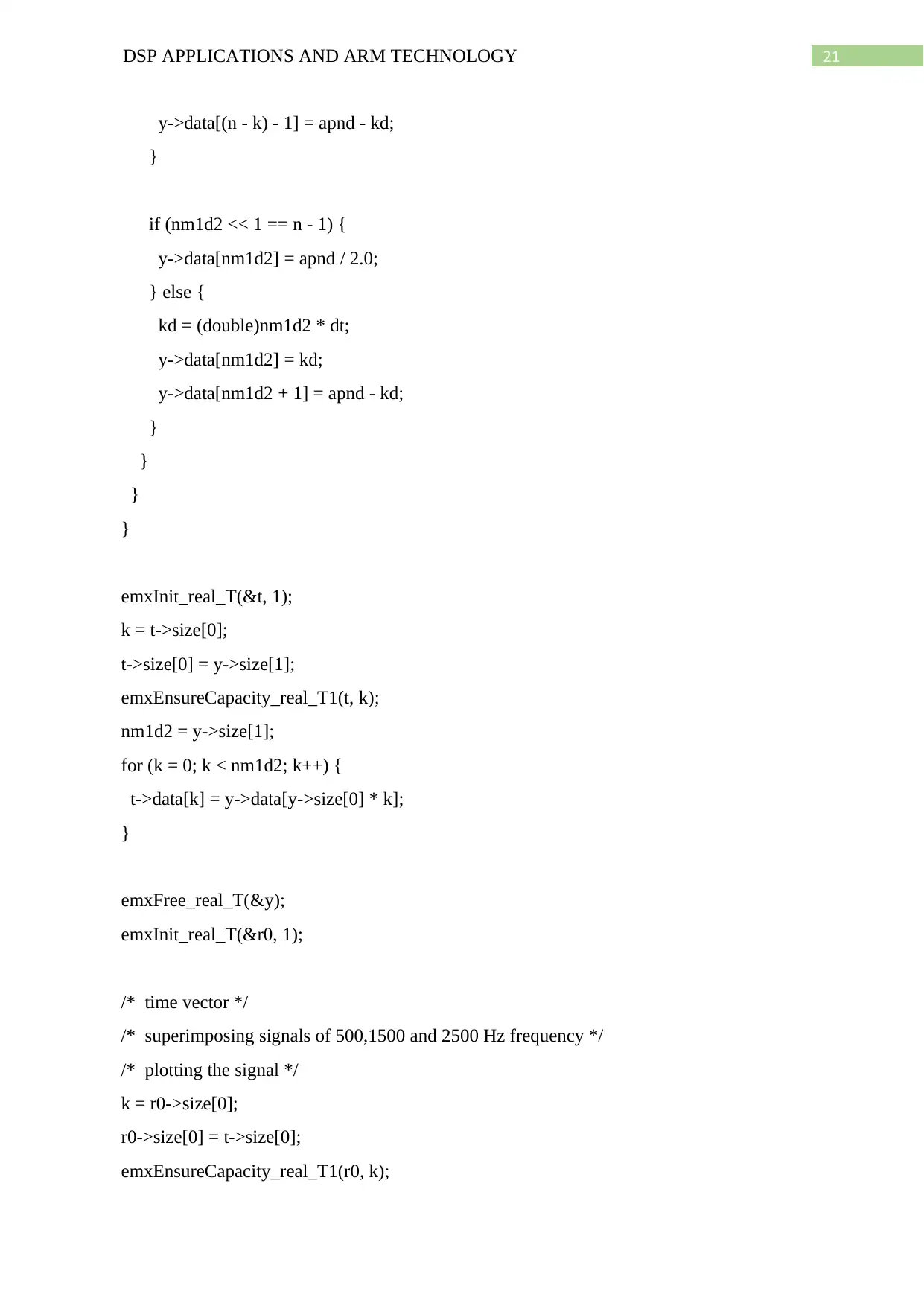
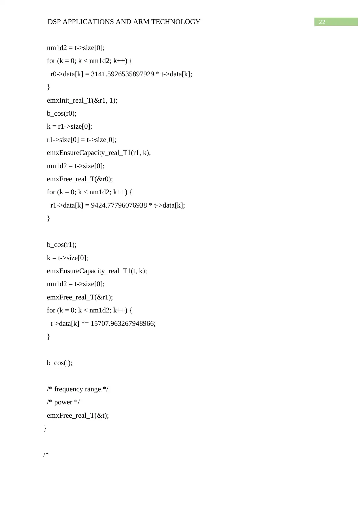
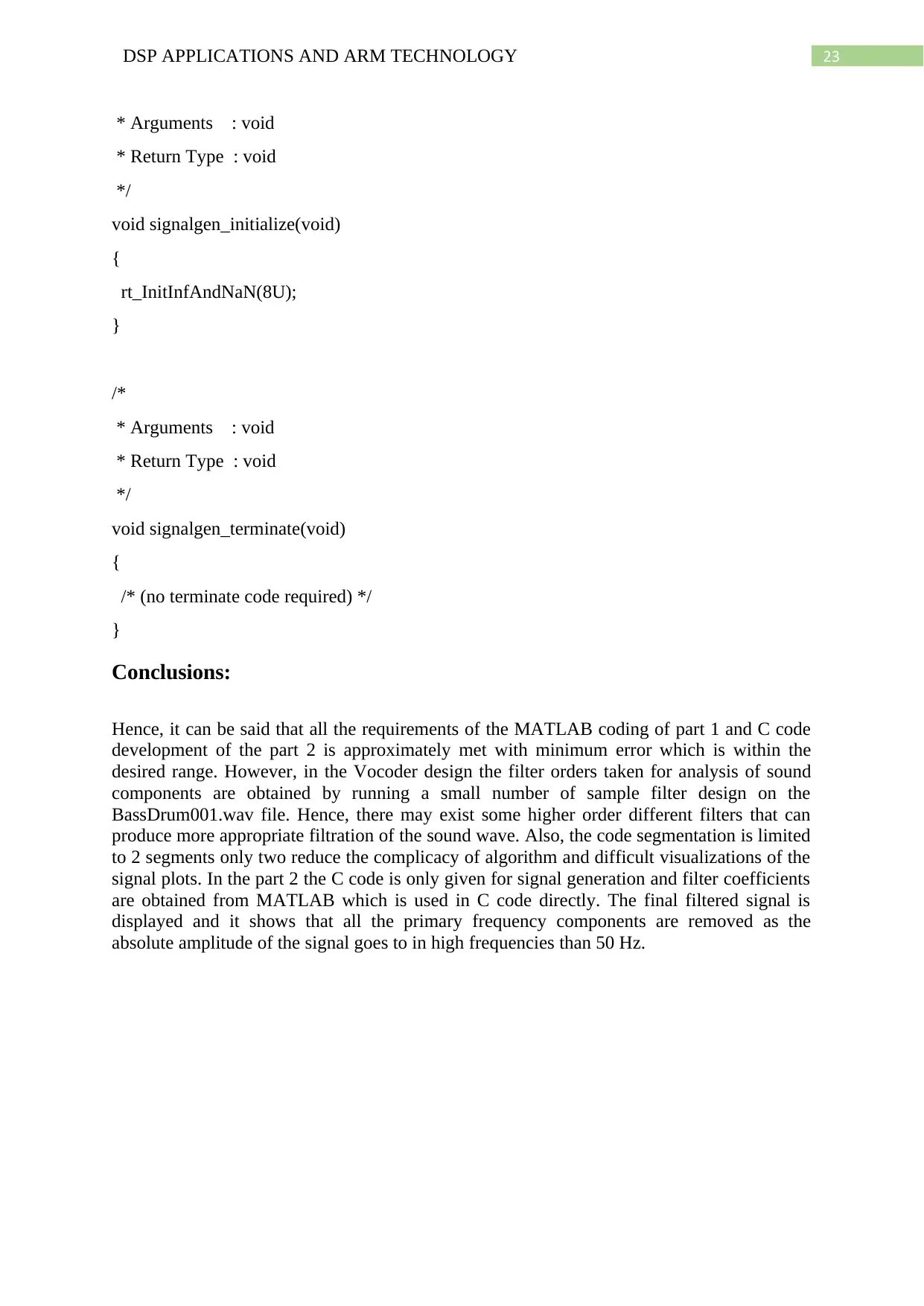
same superposition of three sinusoids can be obtained by the equivalent C code as given
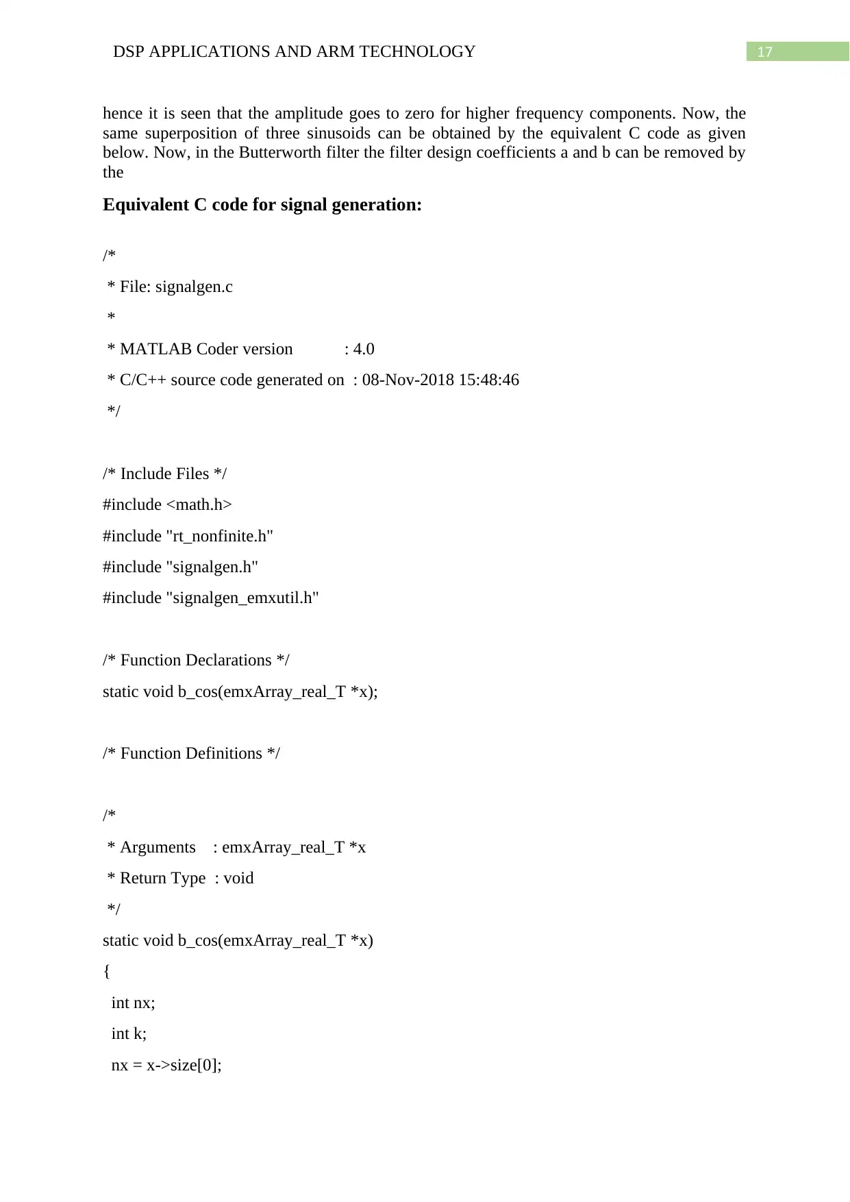
below. Now, in the Butterworth filter the filter design coefficients a and b can be removed by
the
Equivalent C code for signal generation:
/*
* File: signalgen.c
*
* MATLAB Coder version : 4.0
* C/C++ source code generated on : 08-Nov-2018 15:48:46
*/
/* Include Files */
#include <math.h>
#include "rt_nonfinite.h"
#include "signalgen.h"
#include "signalgen_emxutil.h"
/* Function Declarations */
static void b_cos(emxArray_real_T *x);
/* Function Definitions */
/*
* Arguments : emxArray_real_T *x
* Return Type : void
*/
static void b_cos(emxArray_real_T *x)
{
int nx;
int k;
nx = x->size[0];
18DSP APPLICATIONS AND ARM TECHNOLOGY
for (k = 0; k < nx; k++) {
x->data[k] = cos(x->data[k]);
}
}
/*
* Arguments : double Fs
* double stoptime
* Return Type : void
*/
void signalgen(double Fs, double stoptime)
{
emxArray_real_T *y;
double dt;
double kd;
int k;
double ndbl;
double apnd;
emxArray_real_T *t;
double cdiff;
int nm1d2;
int n;
emxArray_real_T *r0;
emxArray_real_T *r1;
emxInit_real_T1(&y, 2);
dt = 1.0 / Fs;
kd = stoptime - dt;
if (rtIsNaN(dt) || rtIsNaN(kd)) {
k = y->size[0] * y->size[1];
y->size[0] = 1;
y->size[1] = 1;
emxEnsureCapacity_real_T(y, k);
Paraphrase This Document
Need a fresh take? Get an instant paraphrase of this document with our AI Paraphraser
19DSP APPLICATIONS AND ARM TECHNOLOGY
y->data[0] = rtNaN;
} else if ((dt == 0.0) || ((0.0 < kd) && (dt < 0.0)) || ((kd < 0.0) && (dt >
0.0))) {
k = y->size[0] * y->size[1];
y->size[0] = 1;
y->size[1] = 0;
emxEnsureCapacity_real_T(y, k);
} else if (rtIsInf(kd) && (rtIsInf(dt) || (0.0 == kd))) {
k = y->size[0] * y->size[1];
y->size[0] = 1;
y->size[1] = 1;
emxEnsureCapacity_real_T(y, k);
y->data[0] = rtNaN;
} else if (rtIsInf(dt)) {
k = y->size[0] * y->size[1];
y->size[0] = 1;
y->size[1] = 1;
emxEnsureCapacity_real_T(y, k);
y->data[0] = 0.0;
} else if (floor(dt) == dt) {
k = y->size[0] * y->size[1];
y->size[0] = 1;
y->size[1] = (int)floor(kd / dt) + 1;
emxEnsureCapacity_real_T(y, k);
nm1d2 = (int)floor(kd / dt);
for (k = 0; k <= nm1d2; k++) {
y->data[y->size[0] * k] = dt * (double)k;
}
} else {
ndbl = floor(kd / dt + 0.5);
apnd = ndbl * dt;
if (dt > 0.0) {
y->data[0] = rtNaN;
} else if ((dt == 0.0) || ((0.0 < kd) && (dt < 0.0)) || ((kd < 0.0) && (dt >
0.0))) {
k = y->size[0] * y->size[1];
y->size[0] = 1;
y->size[1] = 0;
emxEnsureCapacity_real_T(y, k);
} else if (rtIsInf(kd) && (rtIsInf(dt) || (0.0 == kd))) {
k = y->size[0] * y->size[1];
y->size[0] = 1;
y->size[1] = 1;
emxEnsureCapacity_real_T(y, k);
y->data[0] = rtNaN;
} else if (rtIsInf(dt)) {
k = y->size[0] * y->size[1];
y->size[0] = 1;
y->size[1] = 1;
emxEnsureCapacity_real_T(y, k);
y->data[0] = 0.0;
} else if (floor(dt) == dt) {
k = y->size[0] * y->size[1];
y->size[0] = 1;
y->size[1] = (int)floor(kd / dt) + 1;
emxEnsureCapacity_real_T(y, k);
nm1d2 = (int)floor(kd / dt);
for (k = 0; k <= nm1d2; k++) {
y->data[y->size[0] * k] = dt * (double)k;
}
} else {
ndbl = floor(kd / dt + 0.5);
apnd = ndbl * dt;
if (dt > 0.0) {
20DSP APPLICATIONS AND ARM TECHNOLOGY
cdiff = apnd - kd;
} else {
cdiff = kd - apnd;
}
if (fabs(cdiff) < 4.4408920985006262E-16 * fabs(kd)) {
ndbl++;
apnd = kd;
} else if (cdiff > 0.0) {
apnd = (ndbl - 1.0) * dt;
} else {
ndbl++;
}
if (ndbl >= 0.0) {
n = (int)ndbl;
} else {
n = 0;
}
k = y->size[0] * y->size[1];
y->size[0] = 1;
y->size[1] = n;
emxEnsureCapacity_real_T(y, k);
if (n > 0) {
y->data[0] = 0.0;
if (n > 1) {
y->data[n - 1] = apnd;
nm1d2 = (n - 1) / 2;
for (k = 1; k < nm1d2; k++) {
kd = (double)k * dt;
y->data[k] = kd;
21DSP APPLICATIONS AND ARM TECHNOLOGY
y->data[(n - k) - 1] = apnd - kd;
}
if (nm1d2 << 1 == n - 1) {
y->data[nm1d2] = apnd / 2.0;
} else {
kd = (double)nm1d2 * dt;
y->data[nm1d2] = kd;
y->data[nm1d2 + 1] = apnd - kd;
}
}
}
}
emxInit_real_T(&t, 1);
k = t->size[0];
t->size[0] = y->size[1];
emxEnsureCapacity_real_T1(t, k);
nm1d2 = y->size[1];
for (k = 0; k < nm1d2; k++) {
t->data[k] = y->data[y->size[0] * k];
}
emxFree_real_T(&y);
emxInit_real_T(&r0, 1);
/* time vector */
/* superimposing signals of 500,1500 and 2500 Hz frequency */
/* plotting the signal */
k = r0->size[0];
r0->size[0] = t->size[0];
emxEnsureCapacity_real_T1(r0, k);
Secure Best Marks with AI Grader
Need help grading? Try our AI Grader for instant feedback on your assignments.
22DSP APPLICATIONS AND ARM TECHNOLOGY
nm1d2 = t->size[0];
for (k = 0; k < nm1d2; k++) {
r0->data[k] = 3141.5926535897929 * t->data[k];
}
emxInit_real_T(&r1, 1);
b_cos(r0);
k = r1->size[0];
r1->size[0] = t->size[0];
emxEnsureCapacity_real_T1(r1, k);
nm1d2 = t->size[0];
emxFree_real_T(&r0);
for (k = 0; k < nm1d2; k++) {
r1->data[k] = 9424.77796076938 * t->data[k];
}
b_cos(r1);
k = t->size[0];
emxEnsureCapacity_real_T1(t, k);
nm1d2 = t->size[0];
emxFree_real_T(&r1);
for (k = 0; k < nm1d2; k++) {
t->data[k] *= 15707.963267948966;
}
b_cos(t);
/* frequency range */
/* power */
emxFree_real_T(&t);
}
/*
nm1d2 = t->size[0];
for (k = 0; k < nm1d2; k++) {
r0->data[k] = 3141.5926535897929 * t->data[k];
}
emxInit_real_T(&r1, 1);
b_cos(r0);
k = r1->size[0];
r1->size[0] = t->size[0];
emxEnsureCapacity_real_T1(r1, k);
nm1d2 = t->size[0];
emxFree_real_T(&r0);
for (k = 0; k < nm1d2; k++) {
r1->data[k] = 9424.77796076938 * t->data[k];
}
b_cos(r1);
k = t->size[0];
emxEnsureCapacity_real_T1(t, k);
nm1d2 = t->size[0];
emxFree_real_T(&r1);
for (k = 0; k < nm1d2; k++) {
t->data[k] *= 15707.963267948966;
}
b_cos(t);
/* frequency range */
/* power */
emxFree_real_T(&t);
}
/*
23DSP APPLICATIONS AND ARM TECHNOLOGY
* Arguments : void
* Return Type : void
*/
void signalgen_initialize(void)
{
rt_InitInfAndNaN(8U);
}
/*
* Arguments : void
* Return Type : void
*/
void signalgen_terminate(void)
{
/* (no terminate code required) */
}
Conclusions:
Hence, it can be said that all the requirements of the MATLAB coding of part 1 and C code
development of the part 2 is approximately met with minimum error which is within the
desired range. However, in the Vocoder design the filter orders taken for analysis of sound
components are obtained by running a small number of sample filter design on the
BassDrum001.wav file. Hence, there may exist some higher order different filters that can
produce more appropriate filtration of the sound wave. Also, the code segmentation is limited
to 2 segments only two reduce the complicacy of algorithm and difficult visualizations of the
signal plots. In the part 2 the C code is only given for signal generation and filter coefficients
are obtained from MATLAB which is used in C code directly. The final filtered signal is
displayed and it shows that all the primary frequency components are removed as the
absolute amplitude of the signal goes to in high frequencies than 50 Hz.
* Arguments : void
* Return Type : void
*/
void signalgen_initialize(void)
{
rt_InitInfAndNaN(8U);
}
/*
* Arguments : void
* Return Type : void
*/
void signalgen_terminate(void)
{
/* (no terminate code required) */
}
Conclusions:
Hence, it can be said that all the requirements of the MATLAB coding of part 1 and C code
development of the part 2 is approximately met with minimum error which is within the
desired range. However, in the Vocoder design the filter orders taken for analysis of sound
components are obtained by running a small number of sample filter design on the
BassDrum001.wav file. Hence, there may exist some higher order different filters that can
produce more appropriate filtration of the sound wave. Also, the code segmentation is limited
to 2 segments only two reduce the complicacy of algorithm and difficult visualizations of the
signal plots. In the part 2 the C code is only given for signal generation and filter coefficients
are obtained from MATLAB which is used in C code directly. The final filtered signal is
displayed and it shows that all the primary frequency components are removed as the
absolute amplitude of the signal goes to in high frequencies than 50 Hz.
24DSP APPLICATIONS AND ARM TECHNOLOGY
References:
Ahammed, K., Ershadullah, M., Heru, M.R.I., Islam, S. and Sazzad, Z.P., 2015. DESIGN
AND IMPLEMENTATION OF DIGITAL FILTER BANK TO REDUCE NOISE AND
RECONSTRUCT THE INPUT SIGNALS. Signal & Image Processing, 6(2), p.15.
Li, C., Huang, W., Bu, F., Fan, C. and Zhu, P., 2016. Three-Phase Single-Stage AC–DC
Converter Based on Magnetic-Combination Transformer With Power Factor Correction.
IEEE Transactions on Industrial Electronics, 63(12), pp.7320-7327.
Morise, M., Yokomori, F. and Ozawa, K., 2016. WORLD: a vocoder-based high-quality
speech synthesis system for real-time applications. IEICE TRANSACTIONS on Information
and Systems, 99(7), pp.1877-1884.
Podder, P., Hasan, M.M., Islam, M.R. and Sayeed, M., 2014. Design and implementation of
Butterworth, Chebyshev-I and elliptic filter for speech signal analysis. International Journal
of Computer Applications, 98(7).
Sandhu, M., Kaur, S. and Kaur, J., 2016. A study on design and implementation of
Butterworth, Chebyshev and elliptic filter with Matlab. Int. J. Emerg. Technol. Eng. Res,
4(6), pp.111-114.
1 out of 25
Your All-in-One AI-Powered Toolkit for Academic Success.
+13062052269
info@desklib.com
Available 24*7 on WhatsApp / Email
![[object Object]](/_next/static/media/star-bottom.7253800d.svg)
Unlock your academic potential
© 2024 | Zucol Services PVT LTD | All rights reserved.