Dublin Business School Assesment Report
VerifiedAdded on 2022/08/13
|11
|1738
|17
AI Summary
Contribute Materials
Your contribution can guide someone’s learning journey. Share your
documents today.

Dublin Business School
Assessment Brief
1
Assessment Brief
1
Secure Best Marks with AI Grader
Need help grading? Try our AI Grader for instant feedback on your assignments.
Consider a real-world, relational dataset. This dataset must have at least 2 categorical
and 2 continuous variables.
Question 1 (35 Marks)
(a) Describe the dataset using appropriate plots/curves/charts,… (studied 6 plots)
(7)
Sol: code
data<-read.csv("C:\\Users\\George Washington\\Desktop\\save.csv",header=T)
attach(data)
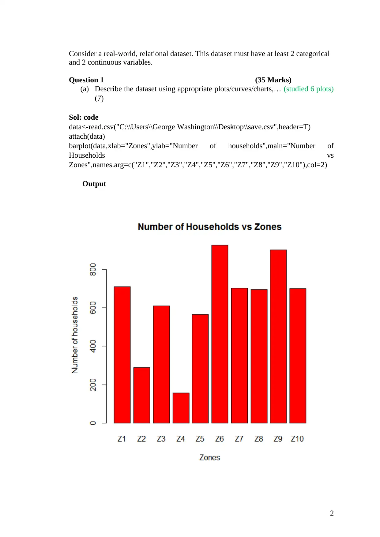
barplot(data,xlab="Zones",ylab="Number of households",main="Number of
Households vs
Zones",names.arg=c("Z1","Z2","Z3","Z4","Z5","Z6","Z7","Z8","Z9","Z10"),col=2)
Output
2
and 2 continuous variables.
Question 1 (35 Marks)
(a) Describe the dataset using appropriate plots/curves/charts,… (studied 6 plots)
(7)
Sol: code
data<-read.csv("C:\\Users\\George Washington\\Desktop\\save.csv",header=T)
attach(data)
barplot(data,xlab="Zones",ylab="Number of households",main="Number of
Households vs
Zones",names.arg=c("Z1","Z2","Z3","Z4","Z5","Z6","Z7","Z8","Z9","Z10"),col=2)
Output
2
data<-read.csv("C:\\Users\\George Washington\\Desktop\\save.csv",header=T)
attach(data)
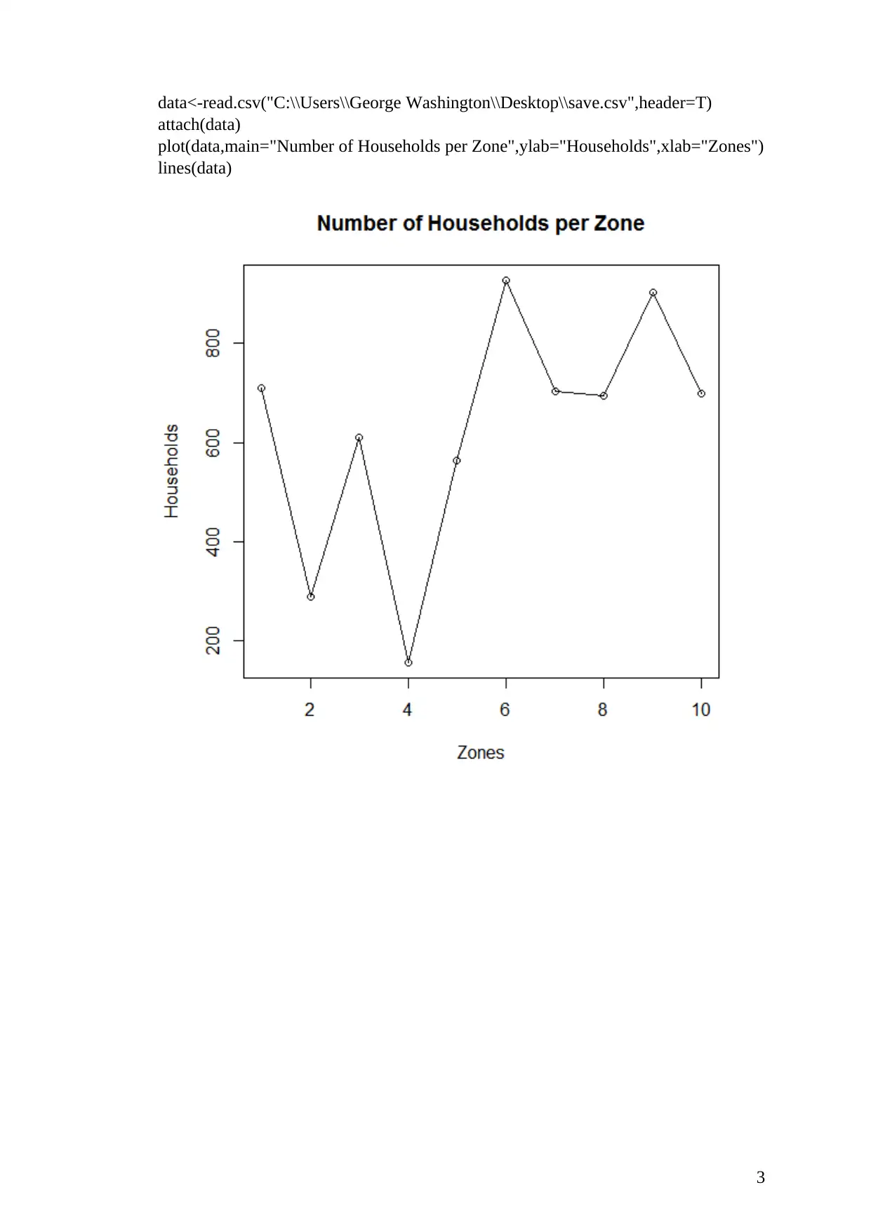
plot(data,main="Number of Households per Zone",ylab="Households",xlab="Zones")
lines(data)
3
attach(data)
plot(data,main="Number of Households per Zone",ylab="Households",xlab="Zones")
lines(data)
3
data<-read.csv("C:\\Users\\George Washington\\Desktop\\save.csv",header=T)
attach(data)
pie(data)
Explanation
The above figure shows the bar graph of the number of households in different zones, that is,
zone 1 – 10.
From the bar graph, it is evident that zone 6 has the highest number of household followed by
zone 9, while zone 4 has the lowest number of households.
Most of the zones have got more than 600 households while only one zone has less than 200
households.
Consider one of continuous attributes, and compute central and variational
measures(. Take mean..take mode..take varience..) (8)
Sol: code
data<-read.csv("C:\\Users\\George Washington\\Desktop\\categorical.csv",header=T)
attach(data)
mean(data)
mode(data)
median(data)
sd(data)
Output
data<-read.csv("C:\\Users\\George Washington\\Desktop\\categorical.csv",header=T)
attach(data)
> mean(data)
[1] 5.372727
> mode(data)
[1] "numeric"
> median(data)
[1] 4
> sd(data)
[1] 2.735723
Explanation
The data is a set of continuous 10 values. The mean is 5.372. This is the average value of the
data. Median is 4. This gives the central value of the data when data is arranged from smallest
4
attach(data)
pie(data)
Explanation
The above figure shows the bar graph of the number of households in different zones, that is,
zone 1 – 10.
From the bar graph, it is evident that zone 6 has the highest number of household followed by
zone 9, while zone 4 has the lowest number of households.
Most of the zones have got more than 600 households while only one zone has less than 200
households.
Consider one of continuous attributes, and compute central and variational
measures(. Take mean..take mode..take varience..) (8)
Sol: code
data<-read.csv("C:\\Users\\George Washington\\Desktop\\categorical.csv",header=T)
attach(data)
mean(data)
mode(data)
median(data)
sd(data)
Output
data<-read.csv("C:\\Users\\George Washington\\Desktop\\categorical.csv",header=T)
attach(data)
> mean(data)
[1] 5.372727
> mode(data)
[1] "numeric"
> median(data)
[1] 4
> sd(data)
[1] 2.735723
Explanation
The data is a set of continuous 10 values. The mean is 5.372. This is the average value of the
data. Median is 4. This gives the central value of the data when data is arranged from smallest
4
Secure Best Marks with AI Grader
Need help grading? Try our AI Grader for instant feedback on your assignments.
to the largest. The standard deviation of the data is 2.73. This gives the deviation about the
mean, the degree by which the data deviates.
(b) For a particular variable of the dataset, use Chebyshev's rule, and propose
one-sigma interval. Select one column calculate sigma..take out outliers
Based on your proposed interval, specify the outliers if any.
(10)
Chebyshev’s rule states that at least 1 – 1/k2 of the data lie within k standard deviations of the
mean, where k is any positive whole number that is greater than 1.
Since k must be positive and greater than one, I propose k = 2. Therefore;
1− 1
4 = 3
4
Hence, three quarters of the data must lie within 2 standard deviations about the mean.
Given this data, therefore;
3.9,7.8,2.7,3.9,4.0,7.2,8.8,2,7,2.3,9.5 with the mean 5.37, three quarters of the data must lie
within 3.37 and 7.37. Thus, according to Chebyshev’s, our data has outliers such as 9.5, 8.8,
2.7 and 7.8.
(c) Explain how the box-plot technique can be used to detect outliers.(different
rules) Apply this technique for one attribute of the dataset (10)
Sol: code
data<-read.csv("C:\\Users\\George Washington\\Desktop\\continuous.csv",header=T)
attach(data)
boxplot(data,main="boxplot")
5
Output
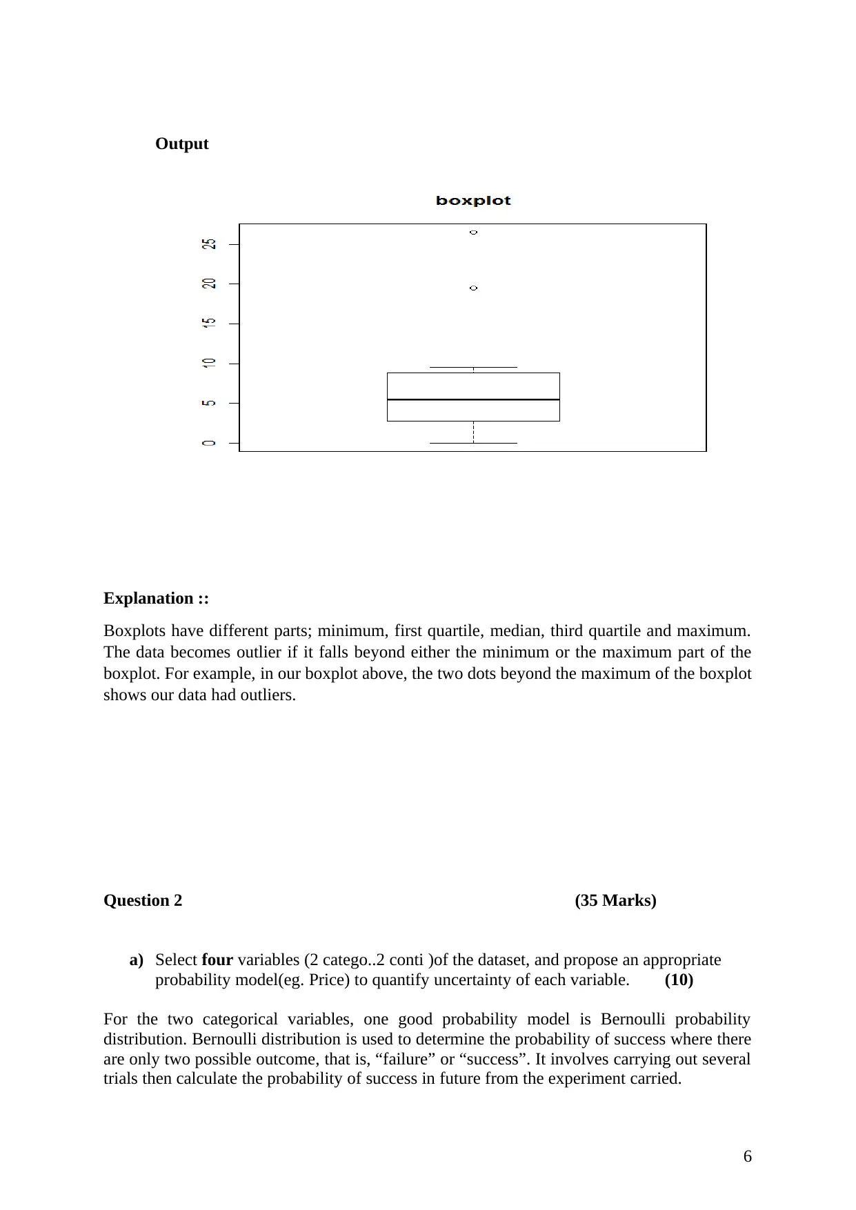
Explanation ::
Boxplots have different parts; minimum, first quartile, median, third quartile and maximum.
The data becomes outlier if it falls beyond either the minimum or the maximum part of the
boxplot. For example, in our boxplot above, the two dots beyond the maximum of the boxplot
shows our data had outliers.
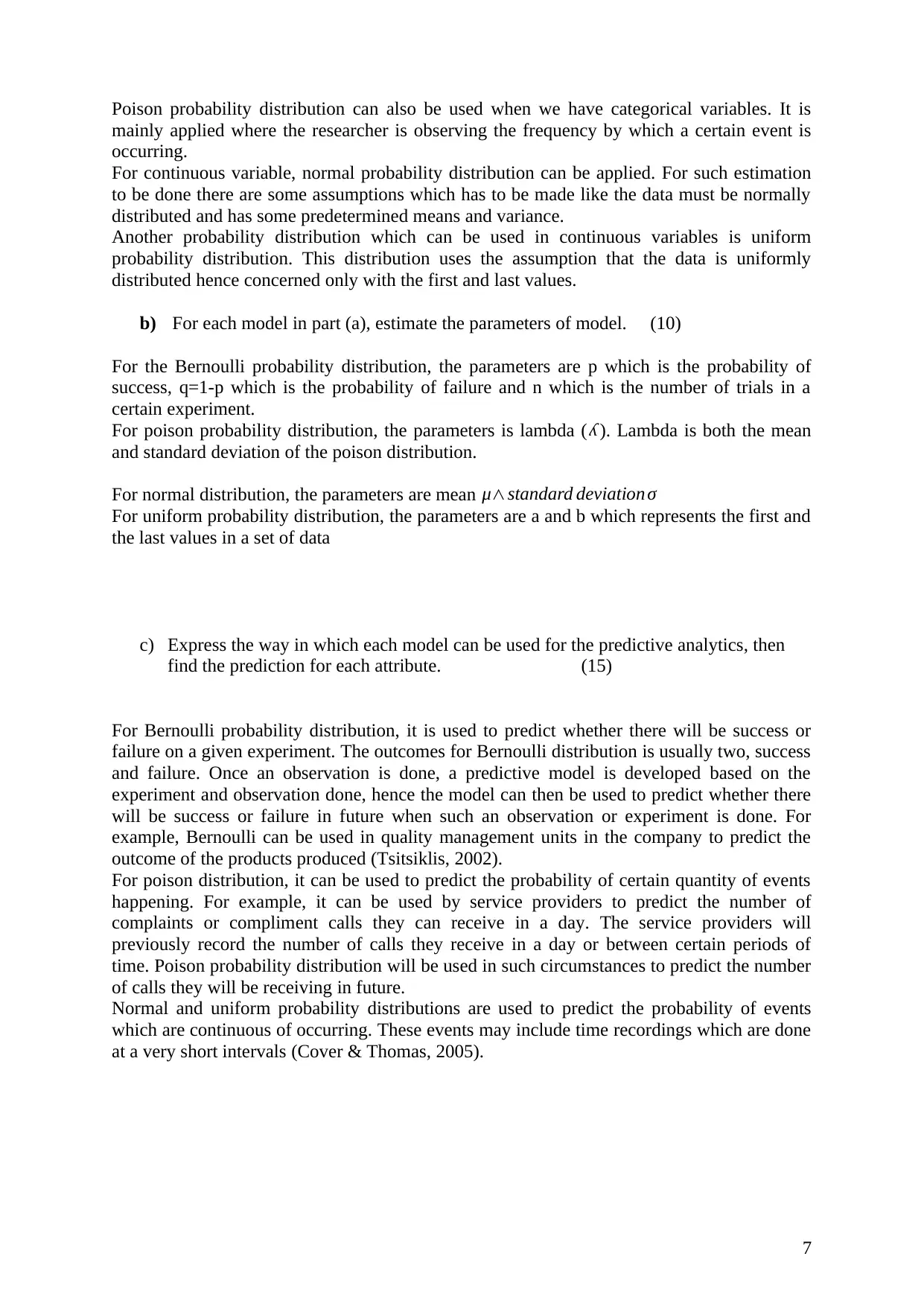
Question 2 (35 Marks)
a) Select four variables (2 catego..2 conti )of the dataset, and propose an appropriate
probability model(eg. Price) to quantify uncertainty of each variable. (10)
For the two categorical variables, one good probability model is Bernoulli probability
distribution. Bernoulli distribution is used to determine the probability of success where there
are only two possible outcome, that is, “failure” or “success”. It involves carrying out several
trials then calculate the probability of success in future from the experiment carried.
6
Explanation ::
Boxplots have different parts; minimum, first quartile, median, third quartile and maximum.
The data becomes outlier if it falls beyond either the minimum or the maximum part of the
boxplot. For example, in our boxplot above, the two dots beyond the maximum of the boxplot
shows our data had outliers.
Question 2 (35 Marks)
a) Select four variables (2 catego..2 conti )of the dataset, and propose an appropriate
probability model(eg. Price) to quantify uncertainty of each variable. (10)
For the two categorical variables, one good probability model is Bernoulli probability
distribution. Bernoulli distribution is used to determine the probability of success where there
are only two possible outcome, that is, “failure” or “success”. It involves carrying out several
trials then calculate the probability of success in future from the experiment carried.
6
Poison probability distribution can also be used when we have categorical variables. It is
mainly applied where the researcher is observing the frequency by which a certain event is
occurring.
For continuous variable, normal probability distribution can be applied. For such estimation
to be done there are some assumptions which has to be made like the data must be normally
distributed and has some predetermined means and variance.
Another probability distribution which can be used in continuous variables is uniform
probability distribution. This distribution uses the assumption that the data is uniformly
distributed hence concerned only with the first and last values.
b) For each model in part (a), estimate the parameters of model. (10)
For the Bernoulli probability distribution, the parameters are p which is the probability of
success, q=1-p which is the probability of failure and n which is the number of trials in a
certain experiment.
For poison probability distribution, the parameters is lambda ( ʎ ). Lambda is both the mean
and standard deviation of the poison distribution.
For normal distribution, the parameters are mean μ∧standard deviation σ
For uniform probability distribution, the parameters are a and b which represents the first and
the last values in a set of data
c) Express the way in which each model can be used for the predictive analytics, then
find the prediction for each attribute. (15)
For Bernoulli probability distribution, it is used to predict whether there will be success or
failure on a given experiment. The outcomes for Bernoulli distribution is usually two, success
and failure. Once an observation is done, a predictive model is developed based on the
experiment and observation done, hence the model can then be used to predict whether there
will be success or failure in future when such an observation or experiment is done. For
example, Bernoulli can be used in quality management units in the company to predict the
outcome of the products produced (Tsitsiklis, 2002).
For poison distribution, it can be used to predict the probability of certain quantity of events
happening. For example, it can be used by service providers to predict the number of
complaints or compliment calls they can receive in a day. The service providers will
previously record the number of calls they receive in a day or between certain periods of
time. Poison probability distribution will be used in such circumstances to predict the number
of calls they will be receiving in future.
Normal and uniform probability distributions are used to predict the probability of events
which are continuous of occurring. These events may include time recordings which are done
at a very short intervals (Cover & Thomas, 2005).
7
Paraphrase This Document
Need a fresh take? Get an instant paraphrase of this document with our AI Paraphraser
Question 3 (30 Marks)
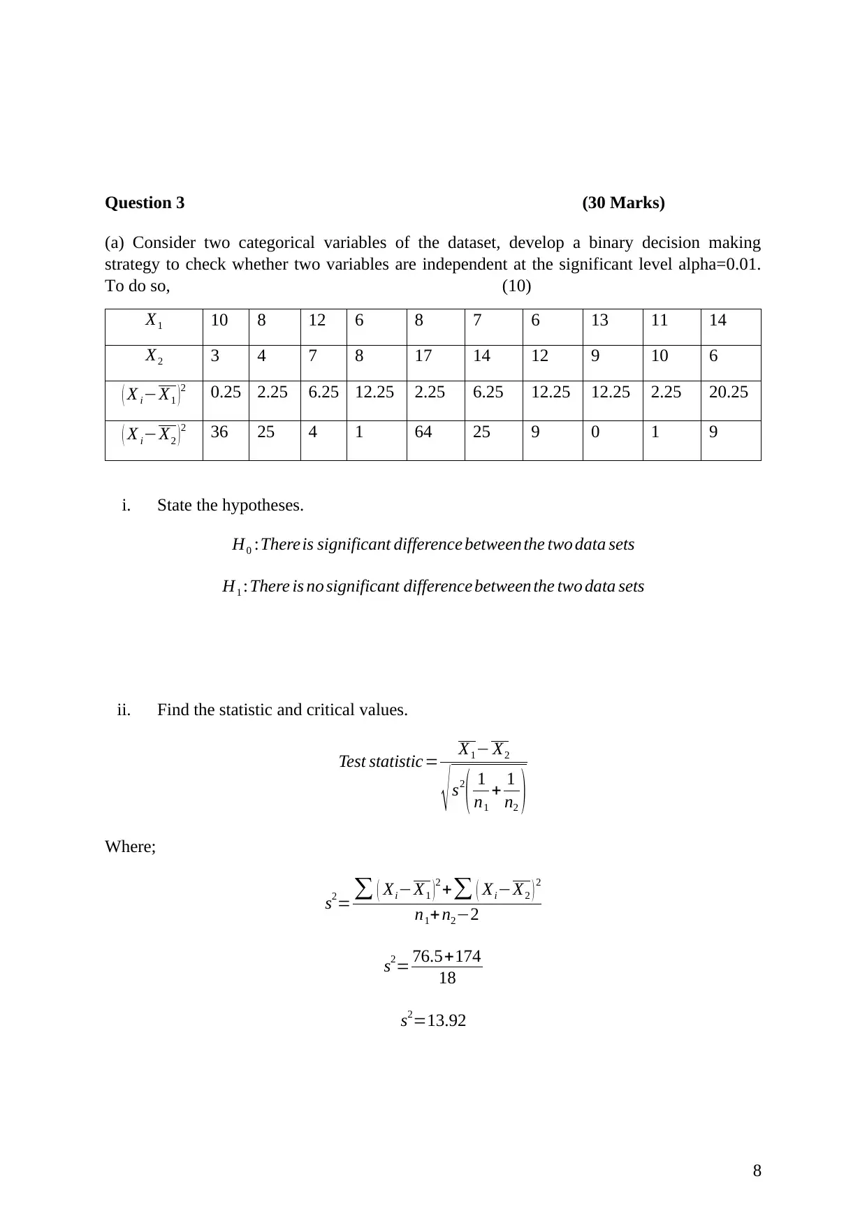
(a) Consider two categorical variables of the dataset, develop a binary decision making
strategy to check whether two variables are independent at the significant level alpha=0.01.
To do so, (10)
X1 10 8 12 6 8 7 6 13 11 14
X2 3 4 7 8 17 14 12 9 10 6
( X i−X1 )2 0.25 2.25 6.25 12.25 2.25 6.25 12.25 12.25 2.25 20.25
( X i−X2 ) 2 36 25 4 1 64 25 9 0 1 9
i. State the hypotheses.
H0 :Thereis significant difference between the two data sets
H1 :There is no significant difference between the two data sets
ii. Find the statistic and critical values.
Test statistic= X1− X2
√s2
( 1
n1
+ 1
n2 )
Where;
s2= ∑ ( Xi−X1 )2 +∑ ( Xi−X2 ) 2
n1+ n2−2
s2= 76.5+174
18
s2=13.92
8
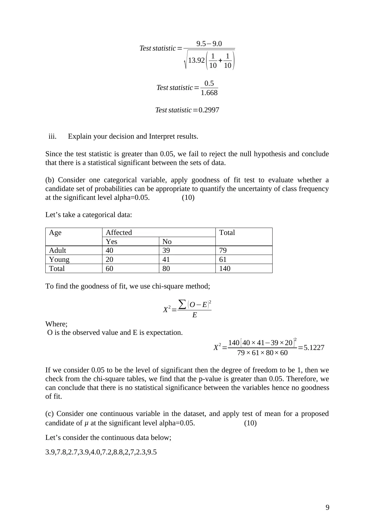
Test statistic= 9.5−9.0
√ 13.92 ( 1
10 + 1
10 )
Test statistic= 0.5
1.668
Test statistic=0.2997
iii. Explain your decision and Interpret results.
Since the test statistic is greater than 0.05, we fail to reject the null hypothesis and conclude
that there is a statistical significant between the sets of data.
(b) Consider one categorical variable, apply goodness of fit test to evaluate whether a
candidate set of probabilities can be appropriate to quantify the uncertainty of class frequency
at the significant level alpha=0.05. (10)
Let’s take a categorical data:
Age Affected Total
Yes No
Adult 40 39 79
Young 20 41 61
Total 60 80 140
To find the goodness of fit, we use chi-square method;
X2 =∑ ( O−E )2
E
Where;
O is the observed value and E is expectation.
X2 =140 [ 40 × 41−39 ×20 ]2
79 × 61× 80× 60 =5.1227
If we consider 0.05 to be the level of significant then the degree of freedom to be 1, then we
check from the chi-square tables, we find that the p-value is greater than 0.05. Therefore, we
can conclude that there is no statistical significance between the variables hence no goodness
of fit.
(c) Consider one continuous variable in the dataset, and apply test of mean for a proposed
candidate of μ at the significant level alpha=0.05. (10)
Let’s consider the continuous data below;
3.9,7.8,2.7,3.9,4.0,7.2,8.8,2,7,2.3,9.5
9
We can test mean by;
z= x−μ
σ
We previously found mean to be 5.37
Therefore, taking μ=4
z= 5.37−4
2.74
z=0.5
Since 0.5 is greater than 0.05 we can then say the mean is not significant at that level
10
z= x−μ
σ
We previously found mean to be 5.37
Therefore, taking μ=4
z= 5.37−4
2.74
z=0.5
Since 0.5 is greater than 0.05 we can then say the mean is not significant at that level
10
Secure Best Marks with AI Grader
Need help grading? Try our AI Grader for instant feedback on your assignments.

References
Cover, T. M., & Thomas, J. A. (2005). Elements of Information Theory. John Wiley and
Sons, 254.
Tsitsiklis, J. N. (2002). Introduction to Probability. Anthena Scientific.
11
Cover, T. M., & Thomas, J. A. (2005). Elements of Information Theory. John Wiley and
Sons, 254.
Tsitsiklis, J. N. (2002). Introduction to Probability. Anthena Scientific.
11
1 out of 11


Your All-in-One AI-Powered Toolkit for Academic Success.
+13062052269
info@desklib.com
Available 24*7 on WhatsApp / Email
![[object Object]](/_next/static/media/star-bottom.7253800d.svg)
Unlock your academic potential
© 2024 | Zucol Services PVT LTD | All rights reserved.