Advanced Electrical Machines and Drives
VerifiedAdded on 2022/11/28
|10
|1193
|362
AI Summary
This document provides study material and solved assignments for Advanced Electrical Machines and Drives. It covers topics such as synchronous speed, speed loop transfer function, HVDC costs, traction motor block diagram, and generator analysis.
Contribute Materials
Your contribution can guide someone’s learning journey. Share your
documents today.
Running head: ADVANCED ELECTRICAL MACHINES AND DRIVES
ADVANCED ELECTRICAL MACHINES AND DRIVES
Name of the Student
Name of the University
Author Note
ADVANCED ELECTRICAL MACHINES AND DRIVES
Name of the Student
Name of the University
Author Note
Secure Best Marks with AI Grader
Need help grading? Try our AI Grader for instant feedback on your assignments.
1DVANCED ELECTRICAL MACHINES AND DRIVES
Question 1:
Given number of poles P = 4, rated speed or rotor speed N = 1706 rpm.
Now, when supplied by 230 volt, 50 Hz source the synchronous speed is
Ns = 120f/P = (120*50)/4 = 1500 rpm.
Slip frequency fs = (N – Ns)*P/2 = (1706 – 1500)*4/2 = 412 rad/sec.
Slip = (N-Ns)/Ns = (1706-1500)/1500 = 0.1373 or 13.73%
Question 2:
The speed loop transfer function is given below,
Fω(s) =
1
1+ s ( 2 D
ωn ) + s2
ωn
2
∗( 1
s )
Here, D = 0.5 and ωn = 314 rad/sec.
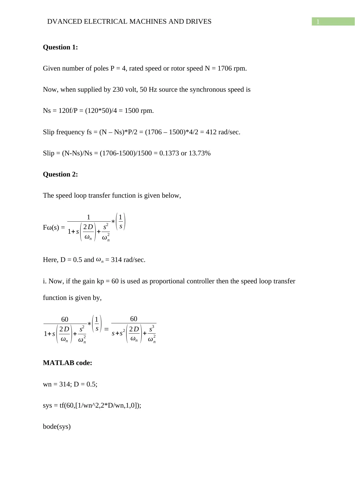
i. Now, if the gain kp = 60 is used as proportional controller then the speed loop transfer
function is given by,
60
1+ s ( 2 D
ωn ) + s2
ωn
2
∗( 1
s ) =
60
s +s2
( 2 D
ωn )+ s3
ωn
2
MATLAB code:
wn = 314; D = 0.5;
sys = tf(60,[1/wn^2,2*D/wn,1,0]);
bode(sys)
Question 1:
Given number of poles P = 4, rated speed or rotor speed N = 1706 rpm.
Now, when supplied by 230 volt, 50 Hz source the synchronous speed is
Ns = 120f/P = (120*50)/4 = 1500 rpm.
Slip frequency fs = (N – Ns)*P/2 = (1706 – 1500)*4/2 = 412 rad/sec.
Slip = (N-Ns)/Ns = (1706-1500)/1500 = 0.1373 or 13.73%
Question 2:
The speed loop transfer function is given below,
Fω(s) =
1
1+ s ( 2 D
ωn ) + s2
ωn
2
∗( 1
s )
Here, D = 0.5 and ωn = 314 rad/sec.
i. Now, if the gain kp = 60 is used as proportional controller then the speed loop transfer
function is given by,
60
1+ s ( 2 D
ωn ) + s2
ωn
2
∗( 1
s ) =
60
s +s2
( 2 D
ωn )+ s3
ωn
2
MATLAB code:
wn = 314; D = 0.5;
sys = tf(60,[1/wn^2,2*D/wn,1,0]);
bode(sys)
2DVANCED ELECTRICAL MACHINES AND DRIVES
Plot:
-100
-80
-60
-40
-20
0
Magnitude (dB)
101 102 103 104
-270
-225
-180
-135
-90
Phase (deg)
Bode Diagram
Frequency (rad/s)
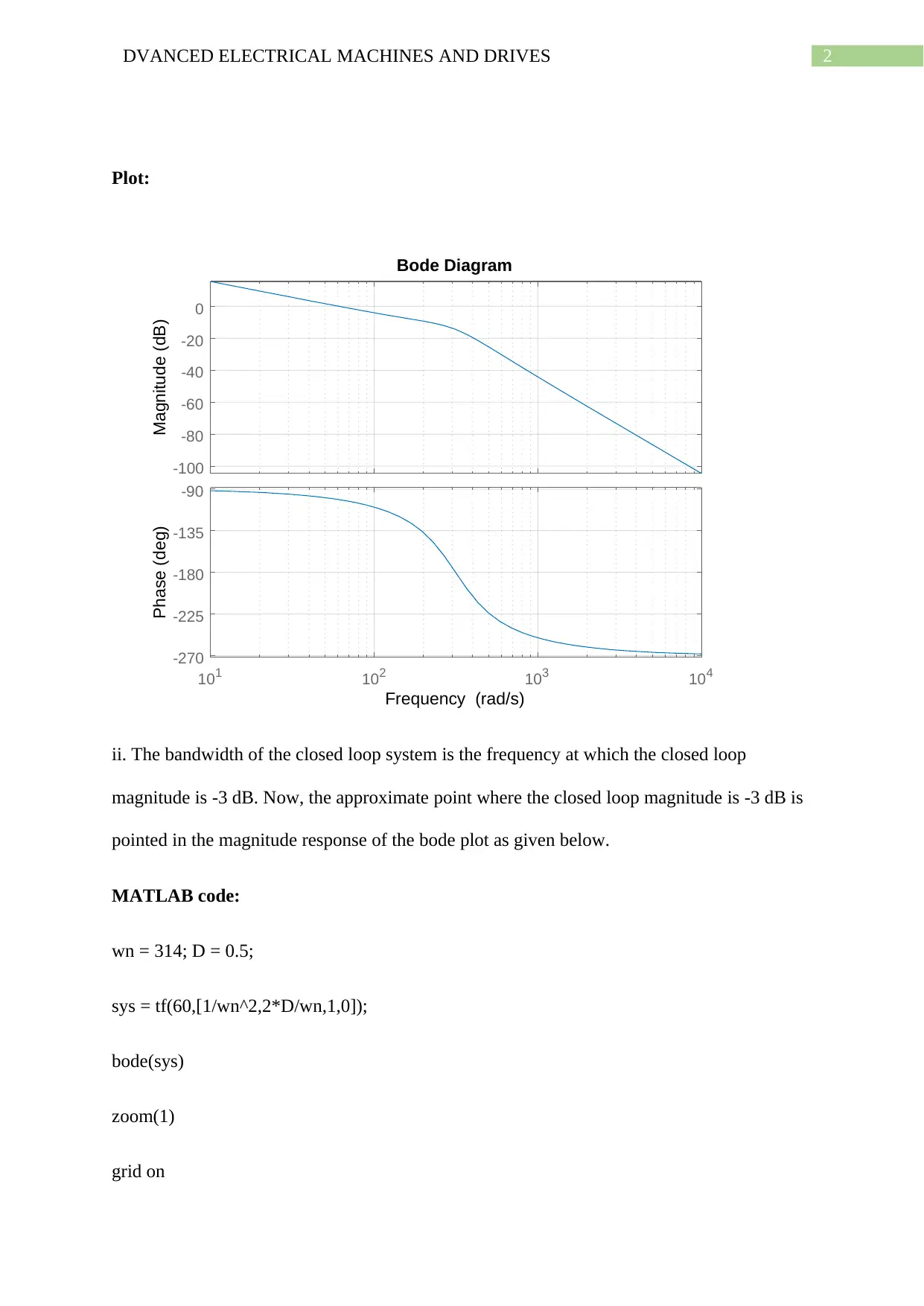
ii. The bandwidth of the closed loop system is the frequency at which the closed loop
magnitude is -3 dB. Now, the approximate point where the closed loop magnitude is -3 dB is
pointed in the magnitude response of the bode plot as given below.
MATLAB code:
wn = 314; D = 0.5;
sys = tf(60,[1/wn^2,2*D/wn,1,0]);
bode(sys)
zoom(1)
grid on
Plot:
-100
-80
-60
-40
-20
0
Magnitude (dB)
101 102 103 104
-270
-225
-180
-135
-90
Phase (deg)
Bode Diagram
Frequency (rad/s)
ii. The bandwidth of the closed loop system is the frequency at which the closed loop
magnitude is -3 dB. Now, the approximate point where the closed loop magnitude is -3 dB is
pointed in the magnitude response of the bode plot as given below.
MATLAB code:
wn = 314; D = 0.5;
sys = tf(60,[1/wn^2,2*D/wn,1,0]);
bode(sys)
zoom(1)
grid on
3DVANCED ELECTRICAL MACHINES AND DRIVES
hold on
[x,y]= ginput(1);
plot(x,y,'ro')
legend('Magnitude response','Bandwidth frequency')
-100
-80
-60
-40
-20
0
Magnitude (dB) Magnitude response
Bandwidth frequency
101 102 103 104
-270
-225
-180
-135
-90
Phase (deg)
Bode Diagram
Frequency (rad/s)
Hence, from the above plot it can be seen that the magnitude response is approximately -3 dB
at the frequency of 90 rad/sec and hence the bandwidth frequency is 90 rad/sec.
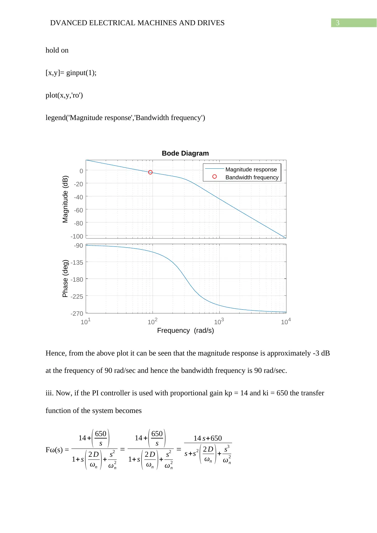
iii. Now, if the PI controller is used with proportional gain kp = 14 and ki = 650 the transfer
function of the system becomes
Fω(s) =
14 +( 650
s )
1+ s ( 2 D
ωn )+ s2
ωn
2
=
14 +( 650
s )
1+ s ( 2 D
ωn )+ s2
ωn
2
=
14 s+650
s +s2
( 2 D
ωn )+ s3
ωn
2
hold on
[x,y]= ginput(1);
plot(x,y,'ro')
legend('Magnitude response','Bandwidth frequency')
-100
-80
-60
-40
-20
0
Magnitude (dB) Magnitude response
Bandwidth frequency
101 102 103 104
-270
-225
-180
-135
-90
Phase (deg)
Bode Diagram
Frequency (rad/s)
Hence, from the above plot it can be seen that the magnitude response is approximately -3 dB
at the frequency of 90 rad/sec and hence the bandwidth frequency is 90 rad/sec.
iii. Now, if the PI controller is used with proportional gain kp = 14 and ki = 650 the transfer
function of the system becomes
Fω(s) =
14 +( 650
s )
1+ s ( 2 D
ωn )+ s2
ωn
2
=
14 +( 650
s )
1+ s ( 2 D
ωn )+ s2
ωn
2
=
14 s+650
s +s2
( 2 D
ωn )+ s3
ωn
2
Secure Best Marks with AI Grader
Need help grading? Try our AI Grader for instant feedback on your assignments.
4DVANCED ELECTRICAL MACHINES AND DRIVES
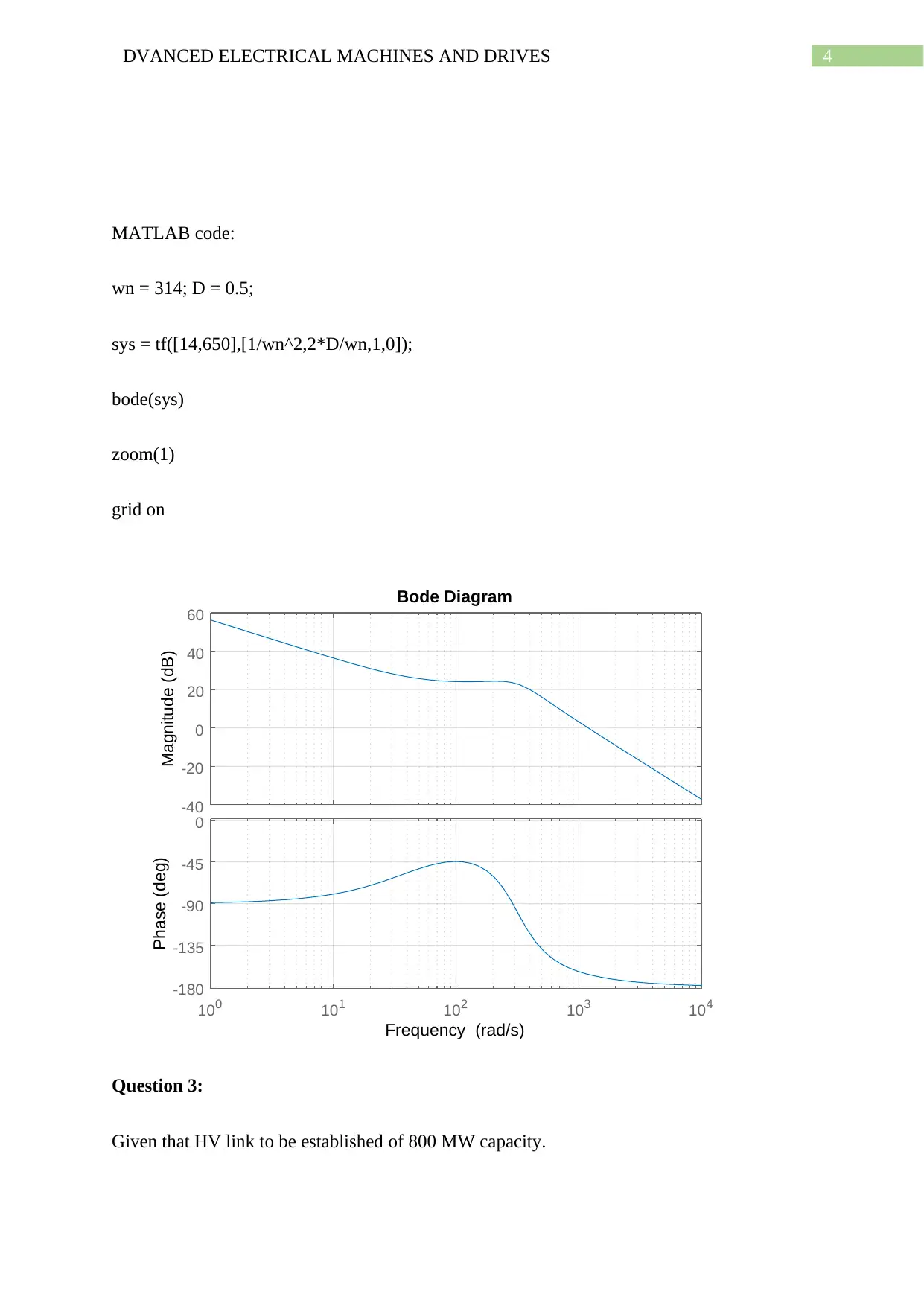
MATLAB code:
wn = 314; D = 0.5;
sys = tf([14,650],[1/wn^2,2*D/wn,1,0]);
bode(sys)
zoom(1)
grid on
-40
-20
0
20
40
60
Magnitude (dB)
100 101 102 103 104
-180
-135
-90
-45
0
Phase (deg)
Bode Diagram
Frequency (rad/s)
Question 3:
Given that HV link to be established of 800 MW capacity.
MATLAB code:
wn = 314; D = 0.5;
sys = tf([14,650],[1/wn^2,2*D/wn,1,0]);
bode(sys)
zoom(1)
grid on
-40
-20
0
20
40
60
Magnitude (dB)
100 101 102 103 104
-180
-135
-90
-45
0
Phase (deg)
Bode Diagram
Frequency (rad/s)
Question 3:
Given that HV link to be established of 800 MW capacity.
5DVANCED ELECTRICAL MACHINES AND DRIVES
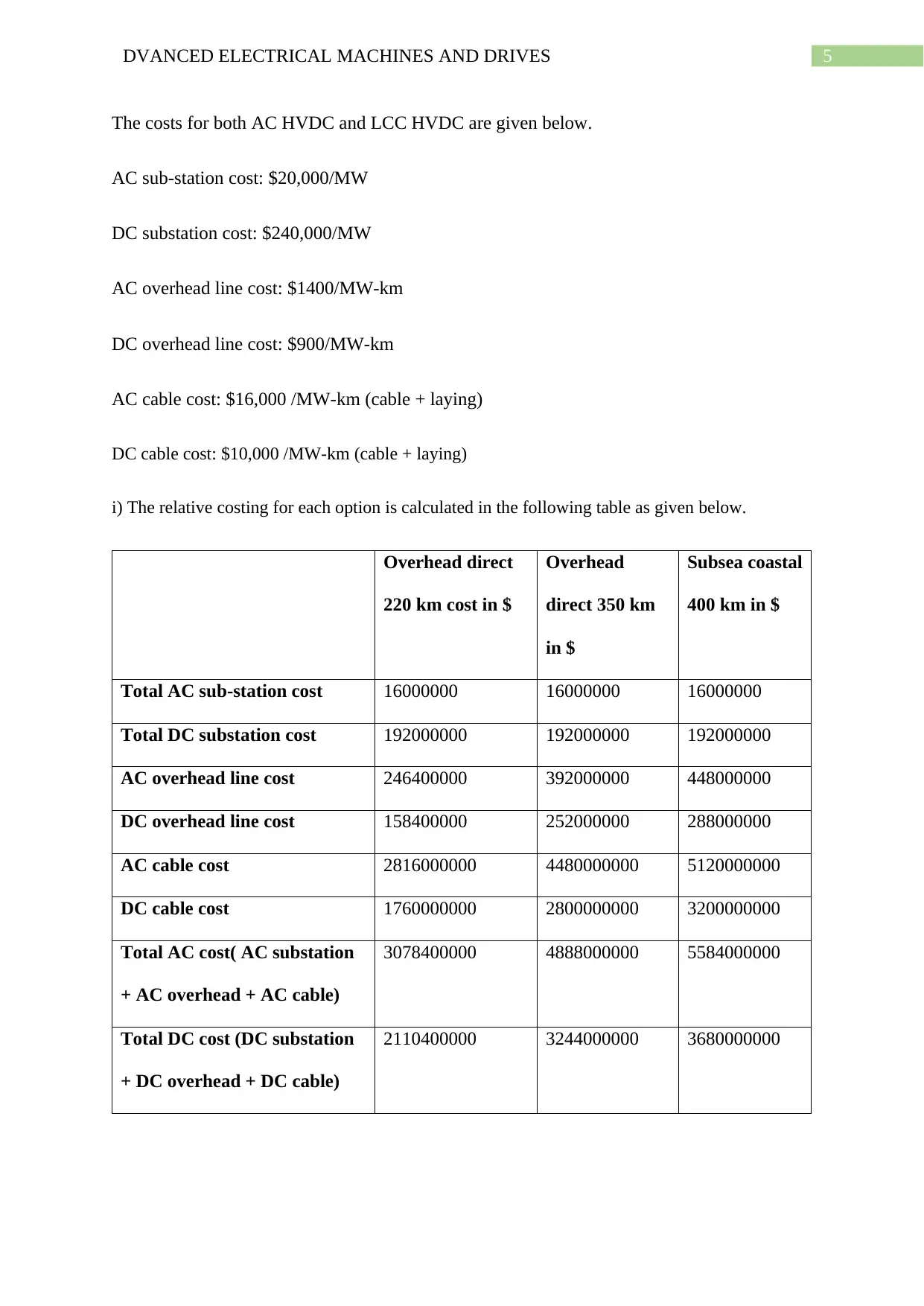
The costs for both AC HVDC and LCC HVDC are given below.
AC sub-station cost: $20,000/MW
DC substation cost: $240,000/MW
AC overhead line cost: $1400/MW-km
DC overhead line cost: $900/MW-km
AC cable cost: $16,000 /MW-km (cable + laying)
DC cable cost: $10,000 /MW-km (cable + laying)
i) The relative costing for each option is calculated in the following table as given below.
Overhead direct
220 km cost in $
Overhead
direct 350 km
in $
Subsea coastal
400 km in $
Total AC sub-station cost 16000000 16000000 16000000
Total DC substation cost 192000000 192000000 192000000
AC overhead line cost 246400000 392000000 448000000
DC overhead line cost 158400000 252000000 288000000
AC cable cost 2816000000 4480000000 5120000000
DC cable cost 1760000000 2800000000 3200000000
Total AC cost( AC substation
+ AC overhead + AC cable)
3078400000 4888000000 5584000000
Total DC cost (DC substation
+ DC overhead + DC cable)
2110400000 3244000000 3680000000
6DVANCED ELECTRICAL MACHINES AND DRIVES
ii. The breakdown distance is the critical distance at which the total AC cost is equal to the
total DC cost.
Now, for option 1 Overhead direct 220 km let the critical distance is x km. Hence, by
breakdown rule
800*20000 + 1400*800*x + 16000*800*x = 800*240000 + 900*800*x + 10000*800*x
x(1400*800 + 16000*800 – 900*800 – 10000*800) = 800(240000-20000)
x(1400 + 16000 – 900 – 10000) = 220000
6500x = 220000 => 33.8462 km.
Similarly for option 2 overhead direct 350 km let the breakdown distance is y km,
800*20000 + 1400*800*y + 16000*800*y = 800*240000 + 900*800*y + 10000*800*y
y = 33.8462 km.
Similarly, for Subsea coastal 400 km the breakdown distance is equal to 33.8462 km.
Hence, the breakdown distance is same for all three options.
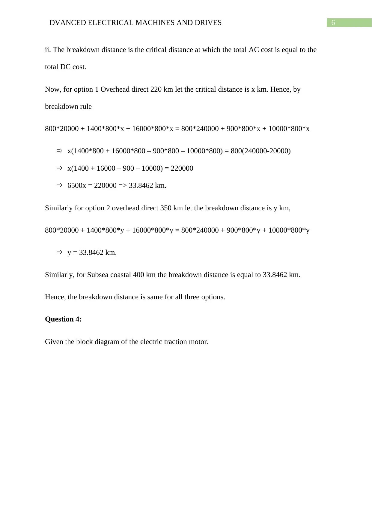
Question 4:
Given the block diagram of the electric traction motor.
ii. The breakdown distance is the critical distance at which the total AC cost is equal to the
total DC cost.
Now, for option 1 Overhead direct 220 km let the critical distance is x km. Hence, by
breakdown rule
800*20000 + 1400*800*x + 16000*800*x = 800*240000 + 900*800*x + 10000*800*x
x(1400*800 + 16000*800 – 900*800 – 10000*800) = 800(240000-20000)
x(1400 + 16000 – 900 – 10000) = 220000
6500x = 220000 => 33.8462 km.
Similarly for option 2 overhead direct 350 km let the breakdown distance is y km,
800*20000 + 1400*800*y + 16000*800*y = 800*240000 + 900*800*y + 10000*800*y
y = 33.8462 km.
Similarly, for Subsea coastal 400 km the breakdown distance is equal to 33.8462 km.
Hence, the breakdown distance is same for all three options.
Question 4:
Given the block diagram of the electric traction motor.
Paraphrase This Document
Need a fresh take? Get an instant paraphrase of this document with our AI Paraphraser
7DVANCED ELECTRICAL MACHINES AND DRIVES
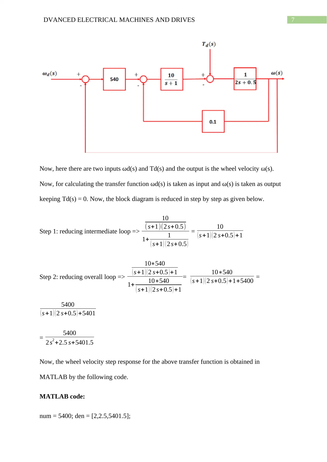
Now, here there are two inputs ωd(s) and Td(s) and the output is the wheel velocity ω(s).
Now, for calculating the transfer function ωd(s) is taken as input and ω(s) is taken as output
keeping Td(s) = 0. Now, the block diagram is reduced in step by step as given below.
Step 1: reducing intermediate loop =>
10
( s+1)(2 s+ 0.5)
1+ 1
( s+1 ) ( 2 s+ 0.5 )
= 10
( s +1 ) ( 2 s+0.5 ) +1
Step 2: reducing overall loop =>
10∗540
( s +1 ) ( 2 s+0.5 )+1
1+ 10∗540
( s+1 ) ( 2 s+0.5 ) +1
= 10∗540
( s +1 ) ( 2 s+0.5 ) +1+5400 =
5400
( s +1 ) ( 2 s+0.5 ) +5401
= 5400
2 s2 +2.5 s+5401.5
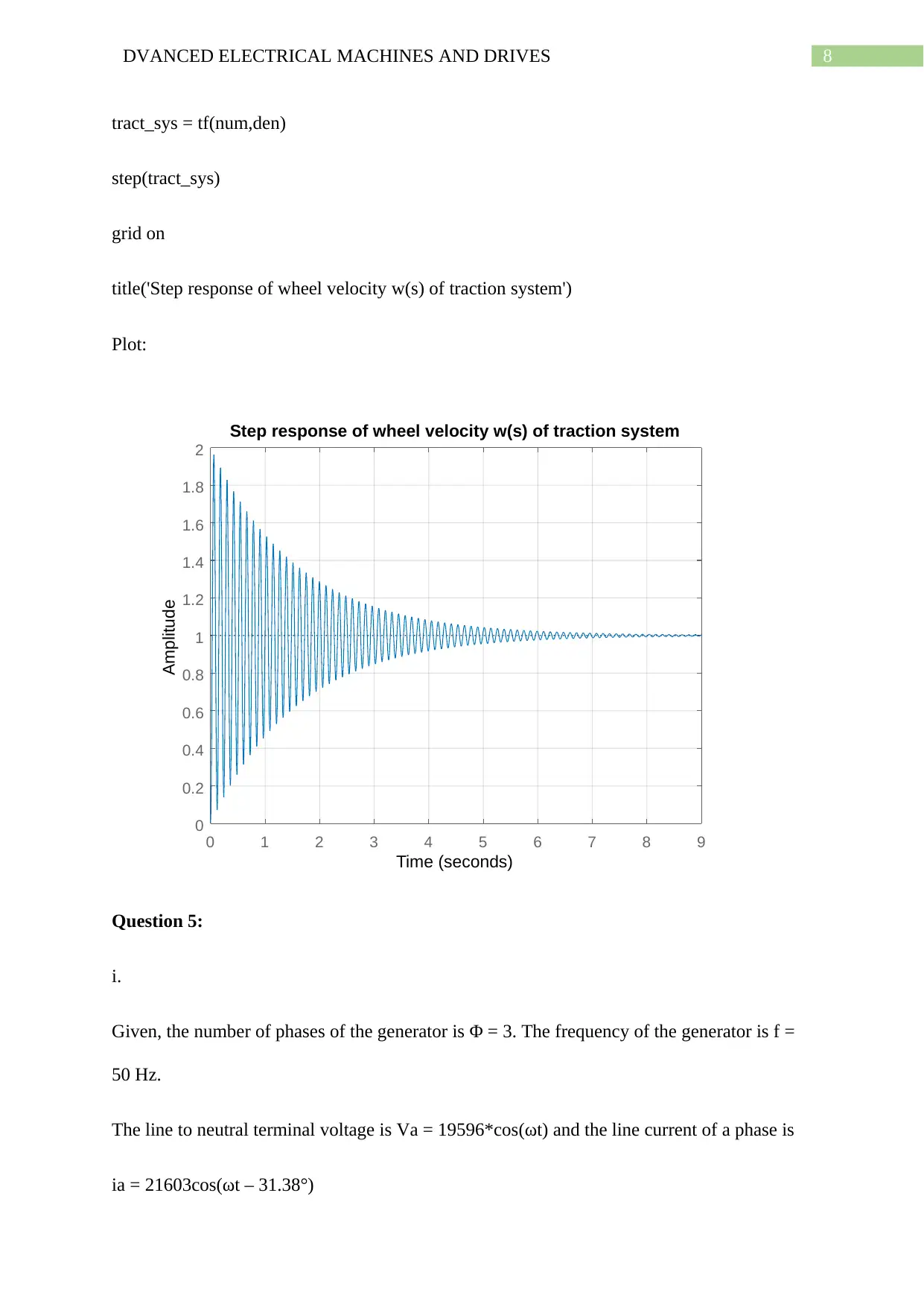
Now, the wheel velocity step response for the above transfer function is obtained in
MATLAB by the following code.
MATLAB code:
num = 5400; den = [2,2.5,5401.5];
Now, here there are two inputs ωd(s) and Td(s) and the output is the wheel velocity ω(s).
Now, for calculating the transfer function ωd(s) is taken as input and ω(s) is taken as output
keeping Td(s) = 0. Now, the block diagram is reduced in step by step as given below.
Step 1: reducing intermediate loop =>
10
( s+1)(2 s+ 0.5)
1+ 1
( s+1 ) ( 2 s+ 0.5 )
= 10
( s +1 ) ( 2 s+0.5 ) +1
Step 2: reducing overall loop =>
10∗540
( s +1 ) ( 2 s+0.5 )+1
1+ 10∗540
( s+1 ) ( 2 s+0.5 ) +1
= 10∗540
( s +1 ) ( 2 s+0.5 ) +1+5400 =
5400
( s +1 ) ( 2 s+0.5 ) +5401
= 5400
2 s2 +2.5 s+5401.5
Now, the wheel velocity step response for the above transfer function is obtained in
MATLAB by the following code.
MATLAB code:
num = 5400; den = [2,2.5,5401.5];
8DVANCED ELECTRICAL MACHINES AND DRIVES
tract_sys = tf(num,den)
step(tract_sys)
grid on
title('Step response of wheel velocity w(s) of traction system')
Plot:
0 1 2 3 4 5 6 7 8 9
0
0.2
0.4
0.6
0.8
1
1.2
1.4
1.6
1.8
2
Step response of wheel velocity w(s) of traction system
Time (seconds)
Amplitude
Question 5:
i.
Given, the number of phases of the generator is Φ = 3. The frequency of the generator is f =
50 Hz.
The line to neutral terminal voltage is Va = 19596*cos(ωt) and the line current of a phase is
ia = 21603cos(ωt – 31.38°)
9DVANCED ELECTRICAL MACHINES AND DRIVES
Hence, the peak voltage at any phase is given by Emax = 19596 volts.
Again, Emax = Nc*Φ*ω, where, Nc = number of conductors at zero degree phase.
19956 = Nc*3*2πf
Nc = 21.1740 ~ 21.
Now, the magnitude of synchronous internal voltage of generator Ea = √2 π∗Nc∗Φ∗f
= √ 2 π∗21∗3∗50 = 13995 volts.
ii.
The total current is given by,
I T=I a +I f
Now, total current is given by,
I T=¿ (MVA rating*10^6)/(rated voltage*10^3*pf) = 645e6/(22e3*0.85) = 34492 Amps.
Now, armature current is I a=21603
Hence, I f = I T - I a = 34492-21603 = 12889 amps.
The flux linkage with the field winding is given by
λf = Lff∗I f + Mf ∗Ia
λf = 433.68e-3*12889 + 31.695e-3*21603 = 6274.4 Wb.
1 out of 10

Your All-in-One AI-Powered Toolkit for Academic Success.
+13062052269
info@desklib.com
Available 24*7 on WhatsApp / Email
![[object Object]](/_next/static/media/star-bottom.7253800d.svg)
Unlock your academic potential
© 2024 | Zucol Services PVT LTD | All rights reserved.