Dynamic Lot Sizing
Added on 2023-01-16
11 Pages2328 Words62 Views
Dynamic Lot Sizing
Introduction
The assignment deals with dynamic lot sizing which is an advanced form of Equilibrium Order
Quantity under which it is understood that demand varies over time and does not remain constant as in
Equilibrium Order Quantity wherein it is assumed that demand remains same throughout the year and
accordingly the order size is determined. The concept of dynamic lot sizing has been introduced by
Harvey M. Wagner and Thomson M.Whitin in 1958 and plays a very vital role in inventory control,
inventory management and cost minimization.
The dynamic lot sizing encompasses season effect of business and plans the business inventory
management strategy accordingly.
Problems
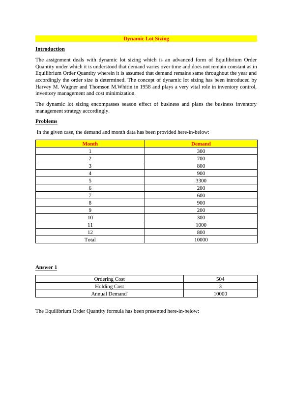
In the given case, the demand and month data has been provided here-in-below:
Month Demand
1 300
2 700
3 800
4 900
5 3300
6 200
7 600
8 900
9 200
10 300
11 1000
12 800
Total 10000
Answer 1
Ordering Cost 504
Holding Cost 3
Annual Demand' 10000
The Equilibrium Order Quantity formula has been presented here-in-below:
Introduction
The assignment deals with dynamic lot sizing which is an advanced form of Equilibrium Order
Quantity under which it is understood that demand varies over time and does not remain constant as in
Equilibrium Order Quantity wherein it is assumed that demand remains same throughout the year and
accordingly the order size is determined. The concept of dynamic lot sizing has been introduced by
Harvey M. Wagner and Thomson M.Whitin in 1958 and plays a very vital role in inventory control,
inventory management and cost minimization.
The dynamic lot sizing encompasses season effect of business and plans the business inventory
management strategy accordingly.
Problems
In the given case, the demand and month data has been provided here-in-below:
Month Demand
1 300
2 700
3 800
4 900
5 3300
6 200
7 600
8 900
9 200
10 300
11 1000
12 800
Total 10000
Answer 1
Ordering Cost 504
Holding Cost 3
Annual Demand' 10000
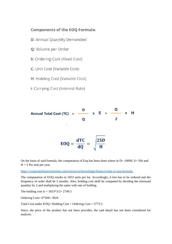
The Equilibrium Order Quantity formula has been presented here-in-below:
On the basis of said formula, the computation of Eoq has been done where in D= 10000, S= 504 and
H = 3 Per unit per year
https://corporatefinanceinstitute.com/resources/knowledge/finance/what-is-eoq-formula/
The computation of EOQ results in 1833 units per lot. Accordingly, 6 lots has to be ordered and the
frequency of order shall be 2 months. Also, holding cost shall be computed by dividing the aforesaid
quantity by 2 and multiplying the same with rate of holding.
The holding cost is = 1833*3/2= 2749.5
Ordering Cost= 6*504= 3024
Total Cost under EOQ= Holding Cost + Ordering Cost = 5773.5
Since, the price of the product has not been provides, the said detail has not been considered for
analysis.
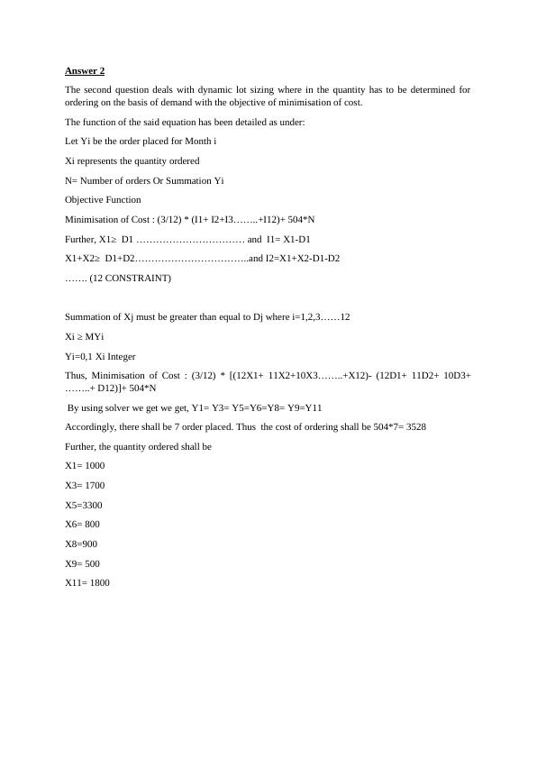
Answer 2
The second question deals with dynamic lot sizing where in the quantity has to be determined for
ordering on the basis of demand with the objective of minimisation of cost.
The function of the said equation has been detailed as under:
Let Yi be the order placed for Month i
Xi represents the quantity ordered
N= Number of orders Or Summation Yi
Objective Function
Minimisation of Cost : (3/12) * (I1+ I2+I3........+I12)+ 504*N
Further, X1≥ D1 ................................. and I1= X1-D1
X1+X2≥ D1+D2...................................and I2=X1+X2-D1-D2
....... (12 CONSTRAINT)
Summation of Xj must be greater than equal to Dj where i=1,2,3......12
Xi ≥ MYi
Yi=0,1 Xi Integer
Thus, Minimisation of Cost : (3/12) * [(12X1+ 11X2+10X3........+X12)- (12D1+ 11D2+ 10D3+
........+ D12)]+ 504*N
By using solver we get we get, Y1= Y3= Y5=Y6=Y8= Y9=Y11
Accordingly, there shall be 7 order placed. Thus the cost of ordering shall be 504*7= 3528
Further, the quantity ordered shall be
X1= 1000
X3= 1700
X5=3300
X6= 800
X8=900
X9= 500
X11= 1800
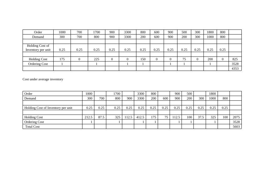
Order 1000 700 1700 900 3300 800 600 900 500 300 1800 800
Demand 300 700 800 900 3300 200 600 900 200 300 1000 800
Holding Cost of
Inventory per unit 0.25 0.25 0.25 0.25 0.25 0.25 0.25 0.25 0.25 0.25 0.25 0.25
Holding Cost 175 0 225 0 0 150 0 0 75 0 200 0 825
Ordering Cost 1 1 1 1 1 1 1 3528
4353
Cost under average inventory
Order 1000 1700 3300 800 900 500 1800
Demand 300 700 800 900 3300 200 600 900 200 300 1000 800
Holding Cost of Inventory per unit 0.25 0.25 0.25 0.25 0.25 0.25 0.25 0.25 0.25 0.25 0.25 0.25
Holding Cost 212.5 87.5 325 112.5 412.5 175 75 112.5 100 37.5 325 100 2075
Ordering Cost 1 1 1 1 1 1 1 3528
Total Cost 5603
Demand 300 700 800 900 3300 200 600 900 200 300 1000 800
Holding Cost of
Inventory per unit 0.25 0.25 0.25 0.25 0.25 0.25 0.25 0.25 0.25 0.25 0.25 0.25
Holding Cost 175 0 225 0 0 150 0 0 75 0 200 0 825
Ordering Cost 1 1 1 1 1 1 1 3528
4353
Cost under average inventory
Order 1000 1700 3300 800 900 500 1800
Demand 300 700 800 900 3300 200 600 900 200 300 1000 800
Holding Cost of Inventory per unit 0.25 0.25 0.25 0.25 0.25 0.25 0.25 0.25 0.25 0.25 0.25 0.25
Holding Cost 212.5 87.5 325 112.5 412.5 175 75 112.5 100 37.5 325 100 2075
Ordering Cost 1 1 1 1 1 1 1 3528
Total Cost 5603
End of preview
Want to access all the pages? Upload your documents or become a member.
Related Documents
Optimal Order Quantity and Total Cost Calculationlg...
|11
|1965
|491
Assignment 1 - Case Studylg...
|6
|1879
|98
Months Demands Received in the Tablelg...
|2
|156
|385
Optimal Order Quantity and Total Cost in Inventory Controllg...
|6
|1041
|44
Inventory Management and Controllg...
|15
|2750
|83