Advanced Modeling, Simulation and Control of Dynamic Systems

This report focuses on the mathematical analysis of the mechanical aspects of the quad bike for the single degree of freedom, two degrees of freedom, and the modeling of the ramp. It includes suitable Laplace Transforms of the modeling equation, transfer function for the system, stability criteria, and bode plot for the system.

Advanced Modeling, Simulation and Control of Dynamic Systems
Student Name
Student ID Number
Institutional Affiliation
Date of Submission
1

2

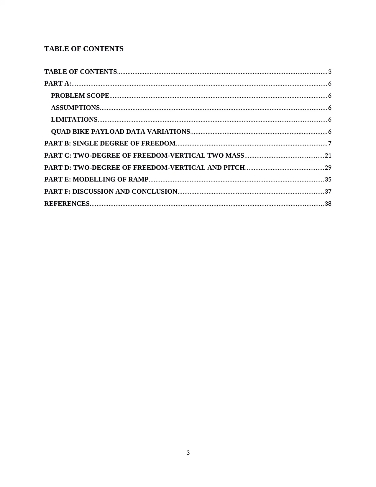
TABLE OF CONTENTS
TABLE OF CONTENTS..........................................................................................................................3
PART A:.....................................................................................................................................................6
PROBLEM SCOPE...............................................................................................................................6
ASSUMPTIONS....................................................................................................................................6
LIMITATIONS.....................................................................................................................................6
QUAD BIKE PAYLOAD DATA VARIATIONS................................................................................6
PART B: SINGLE DEGREE OF FREEDOM........................................................................................7
PART C: TWO-DEGREE OF FREEDOM-VERTICAL TWO MASS..............................................21
PART D: TWO-DEGREE OF FREEDOM-VERTICAL AND PITCH..............................................29
PART E: MODELLING OF RAMP......................................................................................................35
PART F: DISCUSSION AND CONCLUSION.....................................................................................37
REFERENCES........................................................................................................................................38
3

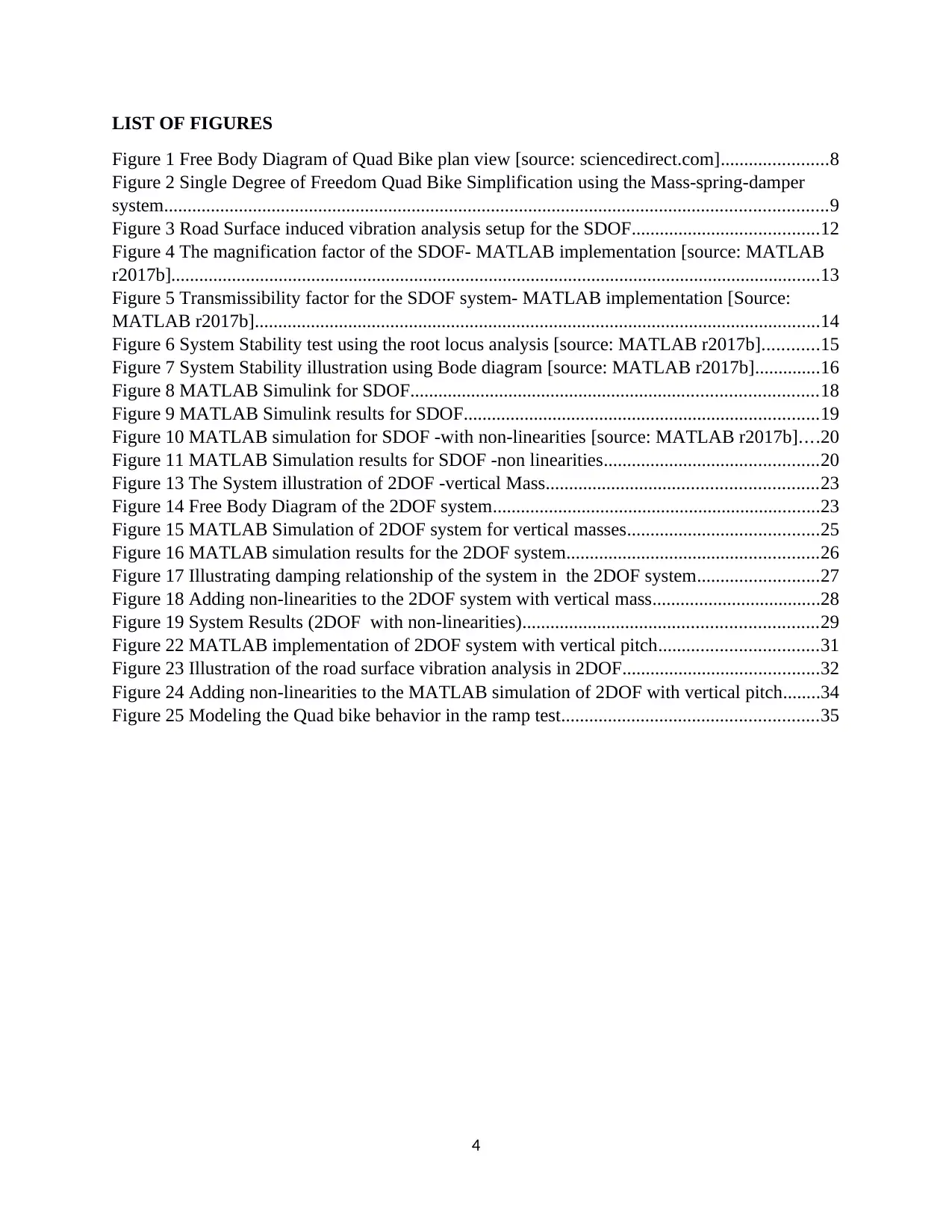
LIST OF FIGURES
Figure 1 Free Body Diagram of Quad Bike plan view [source: sciencedirect.com].......................8
Figure 2 Single Degree of Freedom Quad Bike Simplification using the Mass-spring-damper
system..............................................................................................................................................9
Figure 3 Road Surface induced vibration analysis setup for the SDOF........................................12
Figure 4 The magnification factor of the SDOF- MATLAB implementation [source: MATLAB
r2017b]...........................................................................................................................................13
Figure 5 Transmissibility factor for the SDOF system- MATLAB implementation [Source:
MATLAB r2017b].........................................................................................................................14
Figure 6 System Stability test using the root locus analysis [source: MATLAB r2017b]............15
Figure 7 System Stability illustration using Bode diagram [source: MATLAB r2017b]..............16
Figure 8 MATLAB Simulink for SDOF.......................................................................................18
Figure 9 MATLAB Simulink results for SDOF............................................................................19
Figure 10 MATLAB simulation for SDOF -with non-linearities [source: MATLAB r2017b]....20
Figure 11 MATLAB Simulation results for SDOF -non linearities..............................................20
Figure 13 The System illustration of 2DOF -vertical Mass..........................................................23
Figure 14 Free Body Diagram of the 2DOF system......................................................................23
Figure 15 MATLAB Simulation of 2DOF system for vertical masses.........................................25
Figure 16 MATLAB simulation results for the 2DOF system......................................................26
Figure 17 Illustrating damping relationship of the system in the 2DOF system..........................27
Figure 18 Adding non-linearities to the 2DOF system with vertical mass....................................28
Figure 19 System Results (2DOF with non-linearities)...............................................................29
Figure 22 MATLAB implementation of 2DOF system with vertical pitch..................................31
Figure 23 Illustration of the road surface vibration analysis in 2DOF..........................................32
Figure 24 Adding non-linearities to the MATLAB simulation of 2DOF with vertical pitch........34
Figure 25 Modeling the Quad bike behavior in the ramp test.......................................................35
4

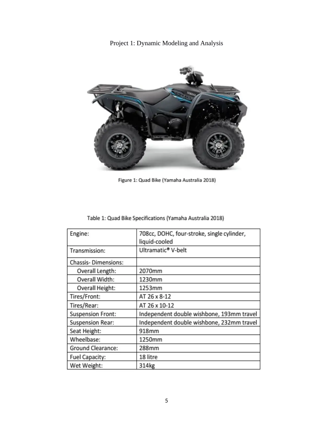
Project 1: Dynamic Modeling and Analysis
5

PART A:
PROBLEM SCOPE
The quad bike analysis seeks to determine the mathematical analysis of the mechanical
aspects of the bike for the single degree of freedom, two degrees of freedom, and the modeling
of the ramp. During analysis, the quad bike is assumed to be implemented on smooth surfaces
with considerable levels of roughness unless where the road roughness is defined. The report
does not focus on the roughness of the road as well as very high degrees of freedom above two
degrees of freedom. Other degrees of freedom are analyzed in other designs to ensure that all
areas that may affect the system.
ASSUMPTIONS
(i) It is assumed that the quad bike has one center of gravity and four wheel of equal height.
(ii) The quad bike has a single rider at every analysis. The chassis and the wheels constitute the
entire weight of the quad bike.
(iii) This is the all-terrain version of Quad bike that operates on the basis of vehicle
propagation for translational and rotary motion. The gravitational acceleration is
given as 9.81 ms-2.
LIMITATIONS
(i) The project is limited to analyzing the quad bike in the single and two-degrees of
freedom.
QUAD BIKE PAYLOAD DATA VARIATIONS
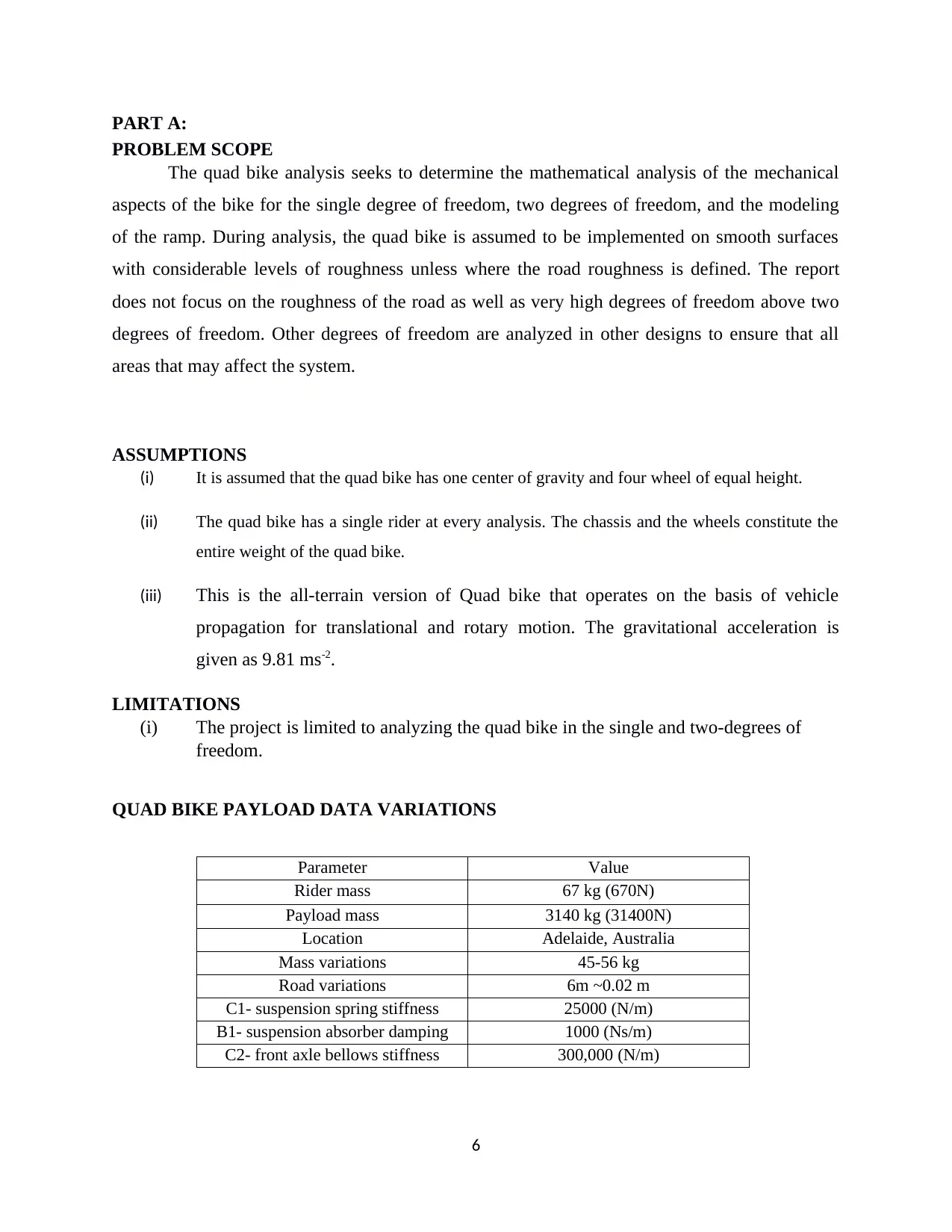
Parameter Value
Rider mass 67 kg (670N)
Payload mass 3140 kg (31400N)
Location Adelaide, Australia
Mass variations 45-56 kg
Road variations 6m ~0.02 m
C1- suspension spring stiffness 25000 (N/m)
B1- suspension absorber damping 1000 (Ns/m)
C2- front axle bellows stiffness 300,000 (N/m)
6

PART B: SINGLE DEGREE OF FREEDOM
Section Goal: To determine the suitable suspension stiffness and damping.
B.1 mathematical model schematic of the quad bike
In this section, the analysis is based on the SDOF analysis of the quad bike. The section seeks to
determine the suitable deferral stiffness and damping. The values obtained for suspension stiffness and
damping are adjusted throughout the analysis to determine the best combination. Mathematical model
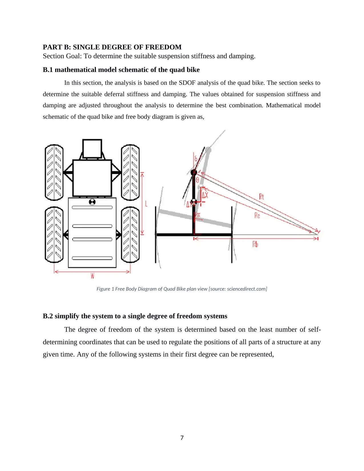
schematic of the quad bike and free body diagram is given as,
Figure 1 Free Body Diagram of Quad Bike plan view [source: sciencedirect.com]
B.2 simplify the system to a single degree of freedom systems
The degree of freedom of the system is determined based on the least number of self-
determining coordinates that can be used to regulate the positions of all parts of a structure at any
given time. Any of the following systems in their first degree can be represented,
7

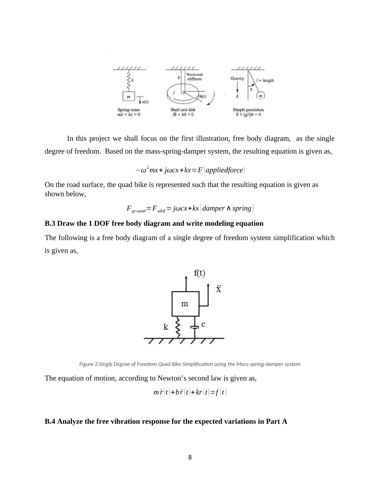
In this project we shall focus on the first illustration, free body diagram, as the single
degree of freedom. Based on the mass-spring-damper system, the resulting equation is given as,
−ω2 mx+ jωcx +kx=F ( appliedforce )
On the road surface, the quad bike is represented such that the resulting equation is given as
shown below,
Fgr ound=Fsdof = jωcx+kx ( damper ∧ spring )
B.3 Draw the 1 DOF free body diagram and write modeling equation
The following is a free body diagram of a single degree of freedom system simplification which
is given as,
Figure 2 Single Degree of Freedom Quad Bike Simplification using the Mass-spring-damper system
The equation of motion, according to Newton’s second law is given as,
m ´r ( t ) +b ´r ( t )+ kr ( t ) =f ( t )
B.4 Analyze the free vibration response for the expected variations in Part A
8

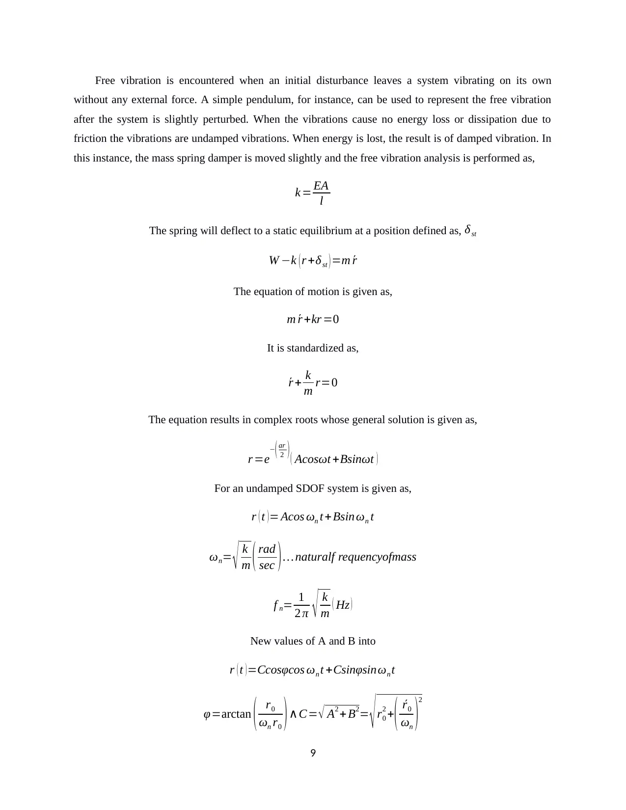
Free vibration is encountered when an initial disturbance leaves a system vibrating on its own
without any external force. A simple pendulum, for instance, can be used to represent the free vibration
after the system is slightly perturbed. When the vibrations cause no energy loss or dissipation due to
friction the vibrations are undamped vibrations. When energy is lost, the result is of damped vibration. In
this instance, the mass spring damper is moved slightly and the free vibration analysis is performed as,
k = EA
l
The spring will deflect to a static equilibrium at a position defined as, δst
W −k ( r +δ st ) =m ´r
The equation of motion is given as,
m ´r +kr =0
It is standardized as,
´r + k
m r=0
The equation results in complex roots whose general solution is given as,
r =e−( ar
2 ) ( Acosωt +Bsinωt )
For an undamped SDOF system is given as,
r ( t ) = Acos ωn t +Bsin ωn t
ωn= √ k
m ( rad
sec )… naturalf requencyofmass
f n= 1
2 π √ k
m ( Hz )
New values of A and B into
r ( t ) =Ccosφcos ωn t +Csinφsinωn t
φ=arctan ( r0
ωn r0 )∧C= √ A2 + B2= √r0
2 +
( ´r0
ωn )2
9

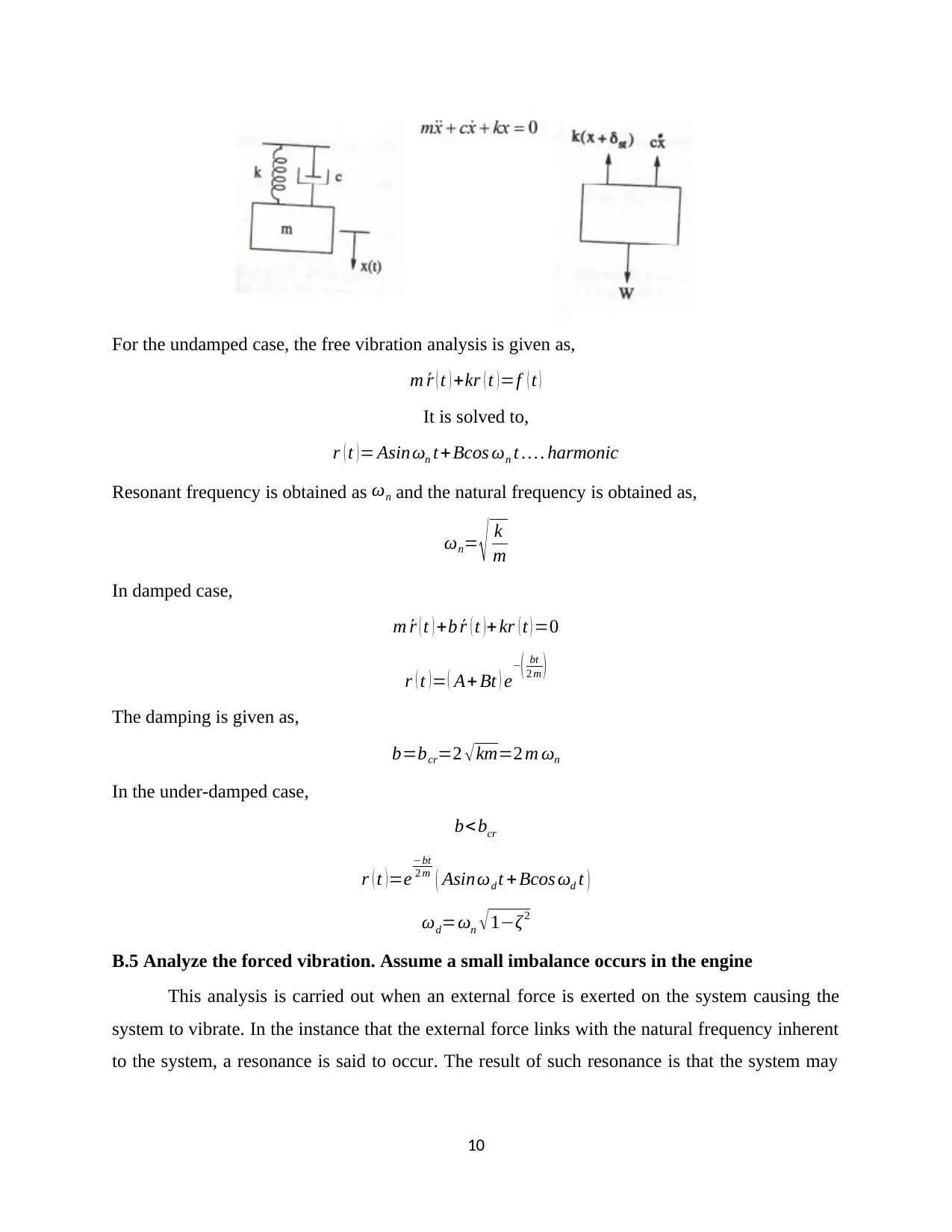
For the undamped case, the free vibration analysis is given as,
m ´r ( t ) +kr ( t ) =f ( t )
It is solved to,
r ( t ) = Asin ωn t+Bcos ωn t … . harmonic
Resonant frequency is obtained as ωn and the natural frequency is obtained as,
ωn= √ k
m
In damped case,
m ´r ( t ) +b ´r ( t )+ kr ( t ) =0
r ( t )= ( A+ Bt ) e−( bt
2 m )
The damping is given as,
b=bcr=2 √ km=2 m ωn
In the under-damped case,
b<bcr
r ( t ) =e
−bt
2 m ( Asinωd t + Bcos ωd t )
ωd=ωn √ 1−ζ2
B.5 Analyze the forced vibration. Assume a small imbalance occurs in the engine
This analysis is carried out when an external force is exerted on the system causing the
system to vibrate. In the instance that the external force links with the natural frequency inherent
to the system, a resonance is said to occur. The result of such resonance is that the system may
10

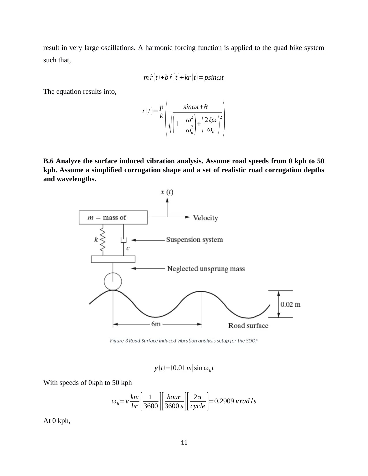
result in very large oscillations. A harmonic forcing function is applied to the quad bike system
such that,
m ´r ( t ) +b ´r ( t ) +kr ( t ) =psinωt
The equation results into,
r ( t )= p
k
( sinωt+θ
√ (1− ω2
ωn
2 )+ (2 ζω
ωn )2
)
B.6 Analyze the surface induced vibration analysis. Assume road speeds from 0 kph to 50
kph. Assume a simplified corrugation shape and a set of realistic road corrugation depths
and wavelengths.
Figure 3 Road Surface induced vibration analysis setup for the SDOF
y ( t ) = ( 0.01 m ) sin ωb t
With speeds of 0kph to 50 kph
ωb=v km
hr [ 1
3600 ][ hour
3600 s ][ 2 π
cycle ]=0.2909 v rad /s
At 0 kph,
11

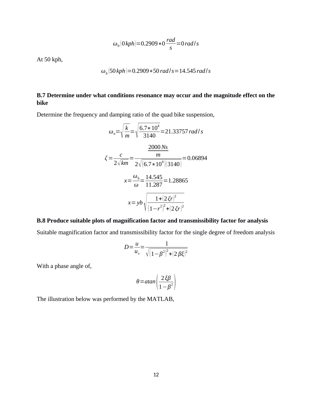
ωb ( 0 kph )=0.2909∗0 rad
s =0 rad /s
At 50 kph,
ωb ( 50 kph ) =0.2909∗50 rad /s=14.545 rad /s
B.7 Determine under what conditions resonance may occur and the magnitude effect on the
bike
Determine the frequency and damping ratio of the quad bike suspension,
ωn= √ k
m= √ 6.7∗104
3140 =21.33757 rad / s
ζ = c
2 √ km =
2000 Ns
m
2 √ ( 6.7∗104 ) ( 3140 ) =0.06894
x= ωb
ω = 14.545
11.287 =1.28865
x= yb
√ 1+ ( 2 ζr )2
( 1−r2 )2
+ ( 2 ζr )2
B.8 Produce suitable plots of magnification factor and transmissibility factor for analysis
Suitable magnification factor and transmissibility factor for the single degree of freedom analysis
D= u
us
= 1
√ ( 1−β2 )
2
+ ( 2 βξ ) 2
With a phase angle of,
θ=atan ( 2 ξβ
1−β2 )
The illustration below was performed by the MATLAB,
12

0 0.5 1 1.5 2 2.5 3
0
2
4
6
8
10
12
E=0.0
E=0.2
E=0.5E=0.7E=1
Figure 4 The magnification factor of the SDOF- MATLAB implementation [source: MATLAB r2017b]
13

0 0.5 1 1.5 2 2.5 3
-2
-1.5
-1
-0.5
0
0.5
1
1.5
2
E=0.0
E=0.2
E=0.5
E=0.7
E=1
Figure 5 Transmissibility factor for the SDOF system- MATLAB implementation [Source: MATLAB r2017b]
B.9 Determine the suitable Laplace Transforms of the modeling equation. Develop a
transfer function for the system and examine the stability criteria and produce a bode plot
for the system. Compare the bode diagrams with plots of magnification factor and
transmissibility factor.
The single degree of freedom Laplace transforms are given by,
L [ f ( t ) ] =F ( s ) =∫
0
∞
f ( t ) e−st dt
m ´r ( t ) +b ´r ( t )+ kr ( t ) … characteristicequation
m s2 R ( s ) +bsR ( s )+ kR ( s )=0
( m s2+bs+k ) R ( s )=0
( m s2+ bs+k )=0 , R ( s ) ≠ 0
T ( s )= 1
3140 s2 + 456 s+ 12.5
14

System stability is determined using the root locus analysis. The root locus analysis is tested
using the pole location on the real axis,
Figure 6 System Stability test using the root locus analysis [source: MATLAB r2017b]
The system stability is demonstrated using the root locus plot. The bode plots are used to
illustrate the magnitude and phase plots.
15

-120
-100
-80
-60
-40
-20
Magnitude (dB)
10 -3 10 -2 10 -1 10 0 10 1
-180
-135
-90
-45
0
Phase (deg)
Bode Diagram
Frequency (rad/s)
Figure 7 System Stability illustration using Bode diagram [source: MATLAB r2017b]
The transmissibility factor and magnification factors plots are obtained using the
following equation with respect to the damping factor,
16

17

B.10 Model the system in Simulink and repeat the analysis on the model. Compare the
Simulink results with the theoretical calculations and explain any differences.
MATLAB Simulation,
Figure 8 MATLAB Simulink for SDOF
Mass = 3140+59=3199 N
Damping coefficient, c = 5.6
18

Spring Stiffness = 6.9
Figure 9 MATLAB Simulink results for SDOF
B.11 Add non-linearities to the spring-mass model in Simulink to make it more reflective of
the real situation [keep the model as a single DOF]. Demonstrate the non-linearities behave
as expected. Repeat the analysis points above where suitable and compare with your
previous results. Draw some conclusions from your comparison.
Some non-linearities were added to the simulation,
19

Figure 10 MATLAB simulation for SDOF -with non-linearities [source: MATLAB r2017b]
Figure 11 MATLAB Simulation results for SDOF -non linearities
20

B.12 Conclusion. State the best suspension stiffness and damping found and summarize
your key findings and observations.
The best suspension stiffness and damping coefficients for the system are as used in the transfer
equation or function. It is given as,
T ( s )= 1
3140 s2 + 456 s+ 12.5
Stiffness= 12.5 N/m
=456 Ns/m
PART C: TWO-DEGREE OF FREEDOM-VERTICAL TWO MASS
C.1 simplify the quad bike system to a two degree of freedom system
It has the yaw and lateral displacement such that the heading velocity is constant with no slope
and body roll. The steering input for the ride is constant and there are lateral accelerations with a
sideslip angle assumed small.
The equation of motion is given as,
m ( ´v +ur )=FF y
+ FR y
I ´r =a FF y
−b F R y
The force that acts on the quad bike tires is given as,
FF y
=Cf α1
FR y
=Cr α 2
α 1=+δ − 1
u ( v +ar ) , α2 =−1
u ( v +br ) , Cf = a
l ,Cr =b
l
Substituting the values in the equation above,
m ( ´v +ur ) =−v
u ( Cf +Cr ) + r
u ( bCr =a Cf ) +δ Cf
21

I ´r =−r
u ( a2 Cf + b2 Cr )− v
u ( a Cf −b Cr ) +aδ Cf
The two-degree system diagram using the bicycle model referencing. The steering angle is
obtained as,
muI ´r + [ I ( Cf +Cr ) ] +m (a2 Cf +b2 Cr ) ´r + ( 1
u ) [ Cf Cr l2−m u2
( a Cf −b Cr ) ] r =mua ( Cf ) ´δ +Cf Cr lδ
Performing the rotational tests or the circle conditions,
´r =0 , ´r=0 , ´δ =0
Then,
r
u [ Cf Cr l2 −mu2
( a Cf −b Cr ) ]=Cf Cr lδ
Further, it is derived as,
+δ= L
R − m v2
Rl ( a
Cr
− b
Cf )
a y= v2
R
When the value is replaced in the equation, we obtain,
δ= L
R − ma y
l ( a
Cr
− b
Cf )
To compute the front slip angle,
+β=−v
u
α 2=−1
u ( v + br )=+β + br
u
+ β=−b
r +α2
22

β=−b
r + αm ay
Cr L
C.2 Draw the simplified model schematic and the 2DOF FBD and write the modeling
equations.
Figure 12 The System illustration of 2DOF -vertical Mass
The 2DOF free body diagram can be demonstrated as shown below,
Figure 13 Free Body Diagram of the 2DOF system
The equation of motion is obtained as,
∑ Forces=−m1 ´x1−c1 ´x1−k1 x1 +k2 ( x2−x1 ) +c2 ( ´x2−´x1 ) + f 1 ( f )=0
For mass 2,
∑ Forces=−m2 ´x2−c2 ( ´x2−´x1 ) −k2 ( x2−x1 )−k 3 x2−c3 ´x2 =0
23

Rearranging the above two expressions of motion with,
m1 ´x1 + ( c1 +c2 ) ´x1 + ( k 1+ k2 ) x1−c2 ´x2−k2 x2=f 1 ( f )
m2 ´x2 + ( c2 +c3 ) ´x2 + ( k2+k3 ) x2−c2 ´x2−k2 x1=0
C.3 from these equations using calculations or MATLAB, determine the free undamped
resonance frequencies and mode shapes. Discuss the meaning of the results with respect to
your aim to analysis of the quad bike.
For the free vibration response analysis,
c2=c1=c3=0
m1 ´x1 + ( k1 + k2 ) x1−k2 x2=f 1 ( f )
m2 ´x2 + ( k 2+k3 ) x2−k2 x1=0
Transforming to Laplace equations
m1 S2 X1 ( s ) + ( k1 +k 2 ) X1 ( s ) −k2 X2 ( s ) =F1 ( s )
m2 S2 X2 ( s ) + ( k 2+ k3 ) X2 ( s ) −k2 X1 ( s ) =0
Where there is no damping,
( m1 S2+ k1 +k2 ) X 1 ( s )−k2 X2 ( s ) =F1 ( s )
( m2 S2 +k2 +k3 ) X2 ( s ) −k2 X1 ( s ) =0
The transfer function is given as,
G1 ( s )= G22 ( s )
G11 x G22 ( s )−G12 ( s ) x G12 ( s )
G1 ( s )= m2 S2 +k2 +k 3
( m1 s2 +k 1+ k2 ) (m2 s2+ k2+ k3 )− (k2 ) ( k 2 )
C.4 Create a suitable 2 DOF Simulink model to also confirm the results
24

Figure 14 MATLAB Simulation of 2DOF system for vertical masses
C.5 using the 2 DOF Simulink model, analyze the road surface induced vibration. Assume
road speeds form 0kph to 50 kph. Assume a simplified corrugation shape and a set of
realistic road corrugation depths and wavelengths.
The results are obtained as,
25

Figure 15 MATLAB simulation results for the 2DOF system
C.6 Create a suitable damped transfer function and use MATLAB scripts to create bode
plots for the damped system undergoing road surface induced vibration.
Where there is no damping,
( m1 S2+ k1 +k2 ) X 1 ( s )−k2 X2 ( s ) =F1 ( s )
( m2 S2 +k2 +k3 ) X2 ( s ) −k2 X1 ( s ) =0
The transfer function is given as,
G1 ( s )= G22 ( s )
G11 x G22 ( s )−G12 ( s ) x G12 ( s )
G1 ( s )= m2 S2 +k2 +k 3
( m1 s2 +k 1+ k2 ) (m2 s2+ k2+ k3 )− (k2 ) ( k 2 )
26

0.05 0.1 0.15 0.2 0.25 0.3 0.35 0.4 0.45 0.5
Frequency (Hz)
10-3
10-2
10-1
100
101
102
Absolute magnitude of G1
Frequency response function of 2DOF-vertical Mass
Figure 16 Illustrating damping relationship of the system in the 2DOF system
C.7 Add non-linearities to the spring mass model in Simulink to make it more reflective of
the real situation. Demonstrate the non-linearities behave as expected.
27

Figure 17 Adding non-linearities to the 2DOF system with vertical mass
28

Figure 18 System Results (2DOF with non-linearities)
C.8 Conclusion. State the best suspension stiffness and damping found and summarize
your key findings and observations.
G ( s ) = 3140 s2 +5.25
1.853∗104 s4 +2.115∗104 s2 +16.13
Stiffness=16.13 N/m
Absorber damper=2.115e4 Ns/m
PART D: TWO-DEGREE OF FREEDOM-VERTICAL AND PITCH
D.1 simplify the quad bike system to a two-degree freedom system (one mass, vertical
motion, and pitch motion)
m ´Z + ( k f +k r ) Z + ( kr c−k f b ) θ=0
´Z+ k f +k r
m Z+ kr c−k f b
m θ=0
´Z+ αZ +βθ=0
m k2 ´θ+ ( k f b2 +k r c2 ) θ+ ( kr c−kf b ) Z=0
29

´θ+ k f b2 +kr c2
mk 2 θ+ k r c−k f b
m k2 Z=0
´θ+ γθ+ β
k2 Z=0
D.2 Estimate the moments of inertia from the diagram and mass data. Check the moment
of inertia value is a realistic value.
The bounce and pitch equations form two differential equations such that,
´Z+ αZ +βθ=0
´θ+ β
k2 Z +γθ=0
β−couplingcoefficient
Z=Zsinωt
θ=θsinωt
Z
θ = β
α −ω2 =−k2 ( γ−ω2 )
β
D.3 Draw a simplified model schematic and the 2 DOF FBD and write modeling equations
( α −ω2 ) ( γ−ω2 )= β2
k2
ω4− ( α + γ ) ω2+ (αγ− β2
k2 )=0
ω1= √ ( α+ γ )
2 + √ ( ( α + γ ) 2
4 ) + β2
k2
ω2= √ ( α + γ )
2 − √ ( ( α +γ ) 2
4 ) + β2
k 2
D.4 calculations or MATLAB to determine the free undamped resonance frequencies and
mode shapes.
The natural frequencies of the front and rear suspensions are defined as,
f f = 1
2 π √ kf g
W f
30

f r= 1
2 π √ k r g
Wr
D.5 Create a suitable 2DOF Simulink model
Figure 19 MATLAB implementation of 2DOF system with vertical pitch
D.6 using the 2DOF Simulink model, analyze the road surface induced vibration. Assume
the road speeds from 0 kph to 50 kph. Assume a simplified corrugation shape and a set of
realistic road corrugation depths and wavelengths.
31

Figure 20 Illustration of the road surface vibration analysis in 2DOF
D.7 Create a suitable damped transfer function and use MATLAB scripts to create bode
plots for the damped system undergoing road surface induced vibration.
Damped Transfer Function,
z ( s )
F ( s ) = 1
m s2 +cs +k =
1
m
s2 + c
m s+ k
m
ωn= k
m … undamednaturalfrequency
Ccr =2 √km … criticaldampingvalue
ζ =amountofproportionald amping
G ( s ) = Z ( s )
F ( s ) = 2.681
s2+ 1.877e06 s+ 1.054 e 2
32

D.8 Add non-linearities to the spring mass model in Simulink to make it more reflective of
the real situation. Demonstrate the non-linearities behave as expected. Repeat the road
analysis and make a conclusion.
33

Figure 21 Adding non-linearities to the MATLAB simulation of 2DOF with vertical pitch
D.9 Conclusion
The suspension stiffness and damping coefficient suitable for use in the two-degree of freedom
in the vertical and pitch,
34

Stiffness = 107.22 N/m
Absorber damper =1.87.756e04 Ns/m
PART E: MODELLING OF RAMP
E.1 Determine and use the best suspension stiffness and damping determined from analysis
in different parts.
Figure 22 Modeling the Quad bike behavior in the ramp test
The best suspension stiffness and damping is determined as,
Stiffness coefficient = 250,000 N/m
Damping coefficient =15,500 Ns/m
35

E.2 Use each Simulink model in parts B, C, and D to get an indication of the quad bike’s
performance over the ramp.
36

E.3 Discuss the free flight behavior of the truck over the jump and the simulation of the
ground contact forces
The quad bike may be tested on a very steep terrain. The system stability depends on how
effectively the center of gravity shifts from the designed position to another to ensure stability
and that that bike does not topple over. The system truck is able to traverse the ramp as long as
the steep angle is less than a certain critical angle as designed.
E.4 Draw conclusions if you were to increase the number of DOF’s how accuracy will be
improved.
The six degrees of freedom are the most accurate for system analysis. The degrees of
freedom are increased to determine the minimal number of coordinates that are considered in the
system analysis. (Kerchmann & Hohman, 2009). The second degree of freedom takes into
consideration more masses than the single degree of freedom.
PART F: DISCUSSION AND CONCLUSION
The project’s main focus was on the suspension stiffness and damping coefficients. It
was determined that the system has different stiffness and damping coefficient for the different
analysis and tests as well as for the single and two degrees of freedom. The system analysis was
illustrated using MATLAB Simulink and further tests on system stability, transmissibility, and
magnitude were carried out. These tests showed that the system is stable based on the location of
poles and the alignment of the magnitude and phase plots. In a nutshell, using multiple degrees
of freedom, allows the designer to evaluate more areas and coordinates of the system than there
are initially.
37

REFERENCES
Kerchmann, V. & Hohman, R. E. T., 2009. Dynamic tire friction models for Quad Bikes
Traction control. Decision and Control: Proceedings of the 38th IEEE conference, 13(4), pp.
3746-3751.
Seoung-On, K. et al., 2012. Actively translating a rear diffuser device for the aerodynamic drag
reduction of a passenger car. International l Journal of Automotive Technology, 13(4), pp. 583-5
38