Motorbike Dynamic System Simulation

This assignment delves into the dynamic modeling and simulation of a motorbike using MATLAB/Simulink. The model considers factors like throttle input, road surface vibrations, and suspension systems. Key analyses include frequency domain representations (Bode plots) and simulations of magnification and transmissibility factors to understand the system's response to external forces.

Dynamic System Modelling and Control

1. Introduction
Several parameters has been controlled the motorbike model development. It has several
criteria. . The simple motorbike implementation associated with 1DOF and vibration analysis is
the major aim of this project. By using Matlab, the motorbike has been implemented. It can be
utilized in all the developments. The several advantages of the motorbike includes safety and
comfort ability. The vibration response and DOF controls the system of dynamic.
2. System of motorbike analysis
Fig 1: motorbike schematic diagram

The motorbike schematic diagram describes the motorbike performance. The throttle is the
input which is given to bike. After that the engine will start and enhance the performance. One
of the power transmission is the torque converter. Mph is the output. The output changes with
respect to speed (DiStefano, Stubberud and Williams, 2014).
3. 1 DOF
It explains the single independent function (co-ordinate).
Fig 2: SDOF in vertical position
The figure explains the 1 DOF vertical position.. Based on the figure, to calculate the
derivations of single degree freedom.
F=m*a
4.Laplace Transform of SDOF:
The Laplace Transform is the method for solving the differential equation and it
converts the time domain equation into algebraic equation which interms of complex variables.
Modelling equation :
----------(1)
The above equation is the Single Degree of Freedom (SDOF).

5.Transfer Function of SDOF:
The transfer function is defined as the ratio of output X(S) to the input F(S).
G(S)=X(S)/F(S)
Fig 3: 1 DOF Transfer Function
Transfer function of the modelling equation:
f(t) f(s)
L(w)=w(s)
L(dw/dt)=sw(s)
L(d2w/dt)=s2w(s)
It gives,
(ms2+cs+k)w(s)=1
W(s)=1/(ms2+cs+k) ---------(2)
The differential equation of laplace transform is,
To find the performance of motorbike in the dynamic system, let us some assumptions are made
for further processing.
The basic weight of the bike (W) is assumed as 250kg. Altitude of the bike (h) is 27.5 inch. Fuel
capacity(c) of the bike is 12.0 liters. Wheel base (Wb) is assumed as 1265 mm. The Front wheel
diameter (Df) is 18 inch, and the rare wheel diameter (Dr) is 18 inch.
W=mg
W=250*9.81

(We assumed g=9.81)
m=2452.5
m=250;
Wf =125; Wr=125
x = ((Wr*Wb) / (Wf+Wr));
x = ((125*1265) / (125+125))
= (158125/250)
= 632.5
W=632.5
In vertical position:
∑ F 1=F1+F2-W=0
6. Simulation of 1DOF:
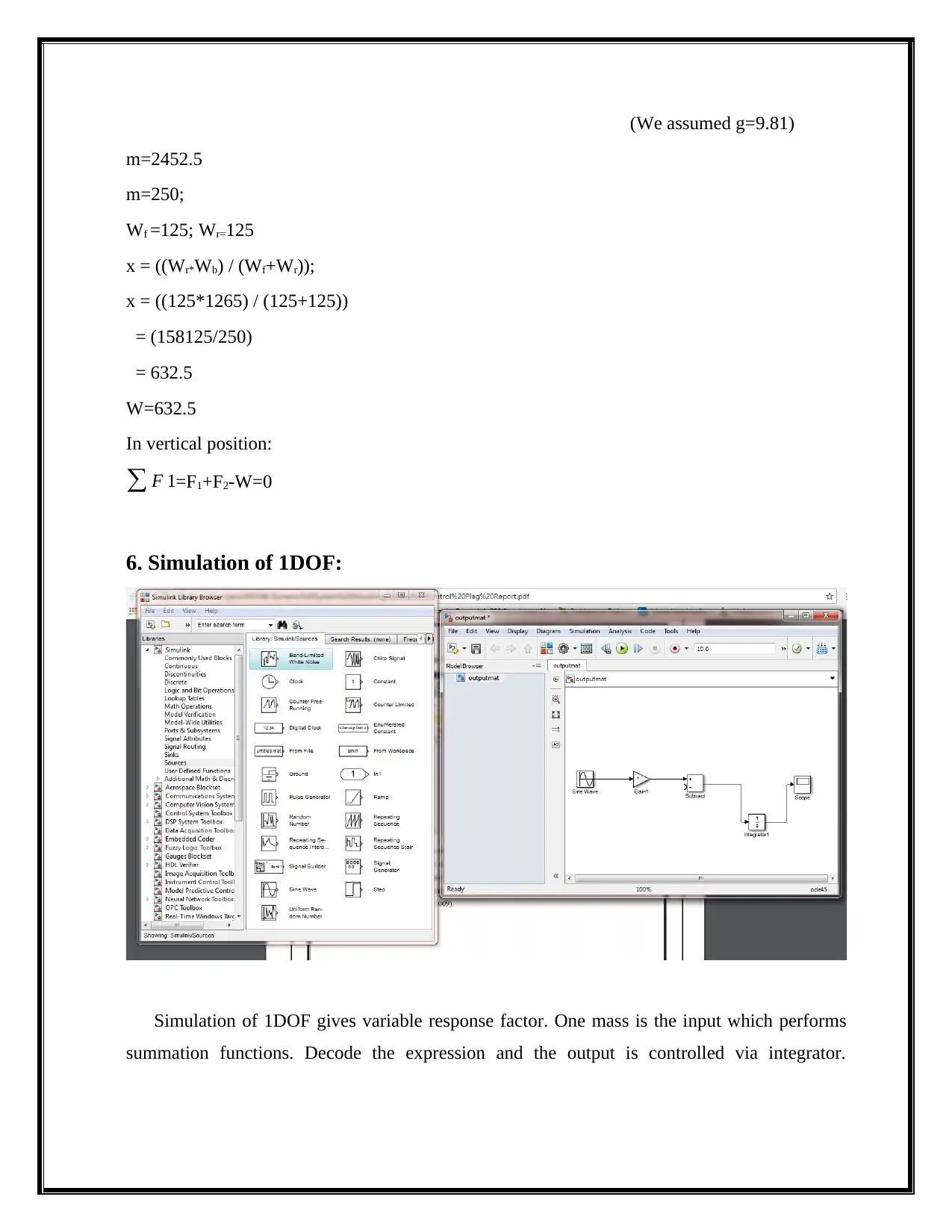
Simulation of 1DOF gives variable response factor. One mass is the input which performs
summation functions. Decode the expression and the output is controlled via integrator.

Therefore, it gives appropriate variable value. After that, simulation was done by Simulink
(Patrick and Fardo, 2009).
7. Output Operation of 1DOF
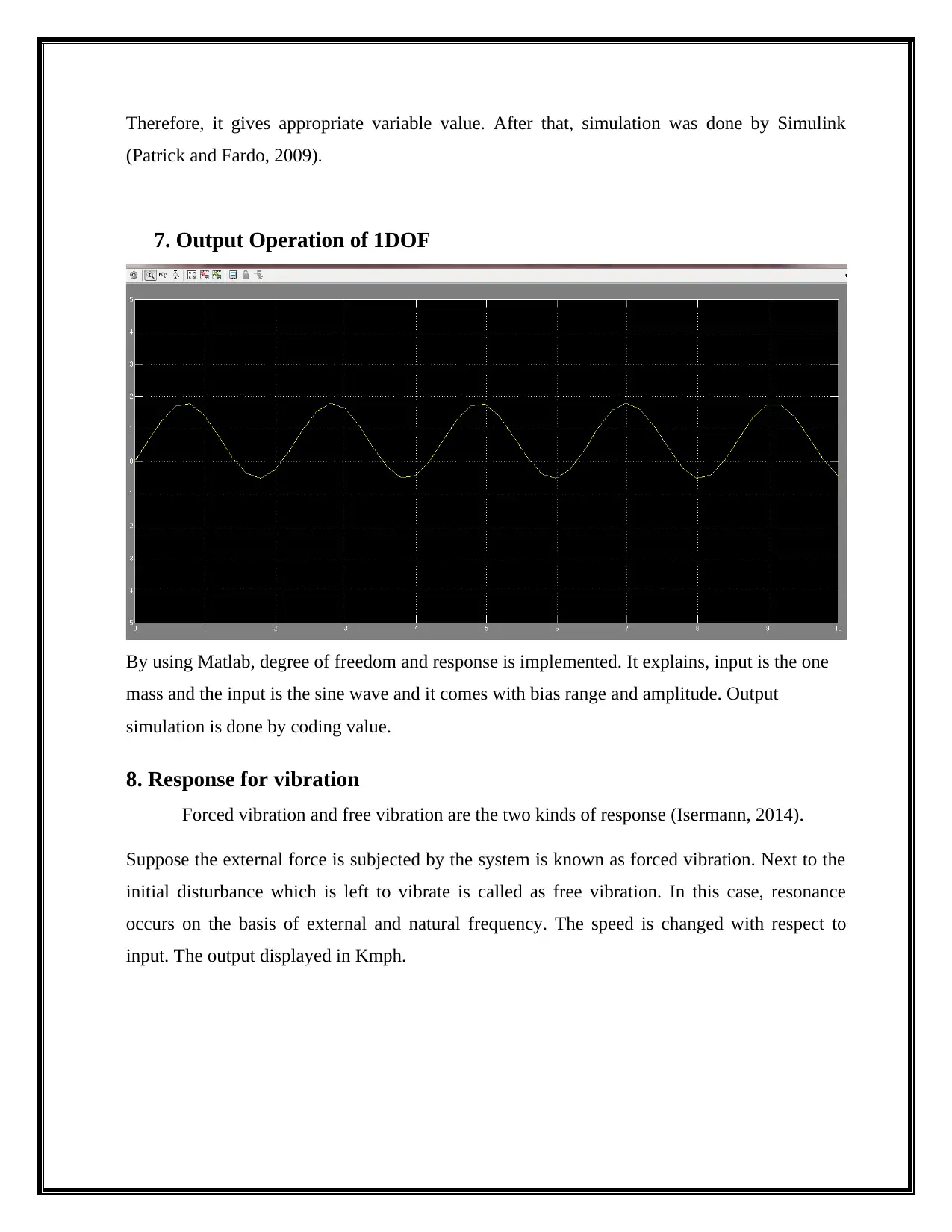
By using Matlab, degree of freedom and response is implemented. It explains, input is the one
mass and the input is the sine wave and it comes with bias range and amplitude. Output
simulation is done by coding value.
8. Response for vibration
Forced vibration and free vibration are the two kinds of response (Isermann, 2014).
Suppose the external force is subjected by the system is known as forced vibration. Next to the
initial disturbance which is left to vibrate is called as free vibration. In this case, resonance
occurs on the basis of external and natural frequency. The speed is changed with respect to
input. The output displayed in Kmph.

Road surface induced vibration
The frictional forces occurs on the road, when riding the motorbike. The longitudinal angle is
defined as the ratio between the angle velocity to the forward velocity. The motorbike is
represented by an angle which is less than 90 degree. Because the motorbike is no longer in
perpendicular position to the road surface.
9. Simulation of Vibration
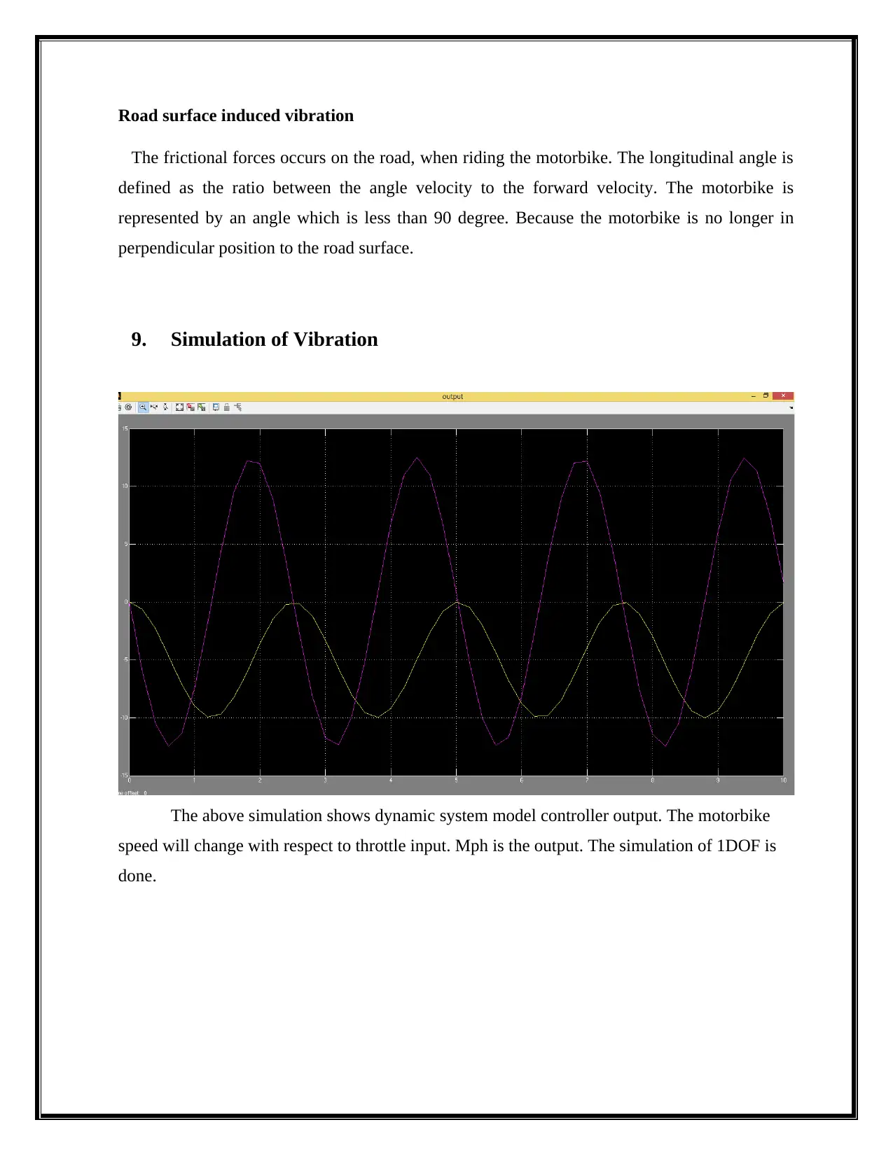
The above simulation shows dynamic system model controller output. The motorbike
speed will change with respect to throttle input. Mph is the output. The simulation of 1DOF is
done.

10. Plot of Magnification Factor and Transmissibility factor
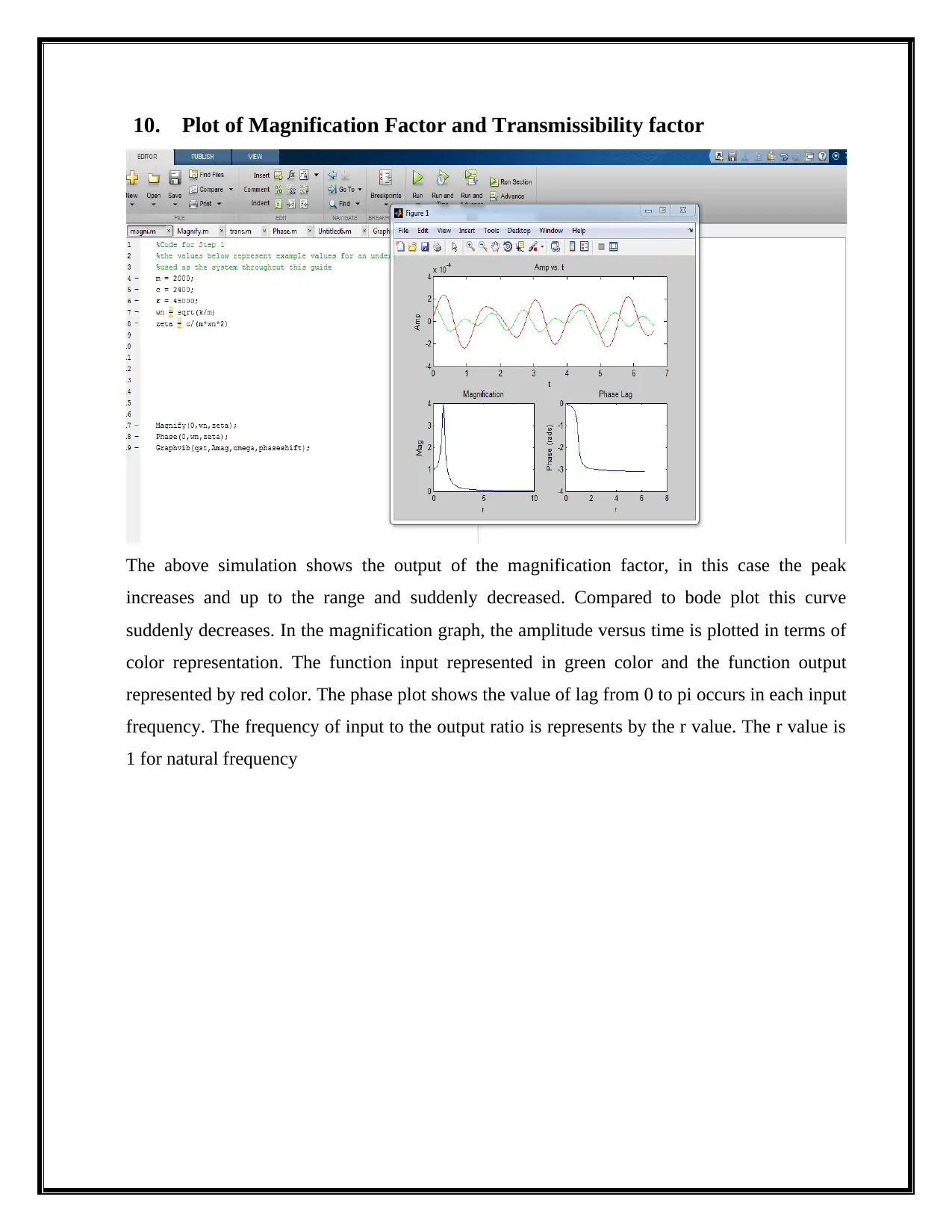
The above simulation shows the output of the magnification factor, in this case the peak
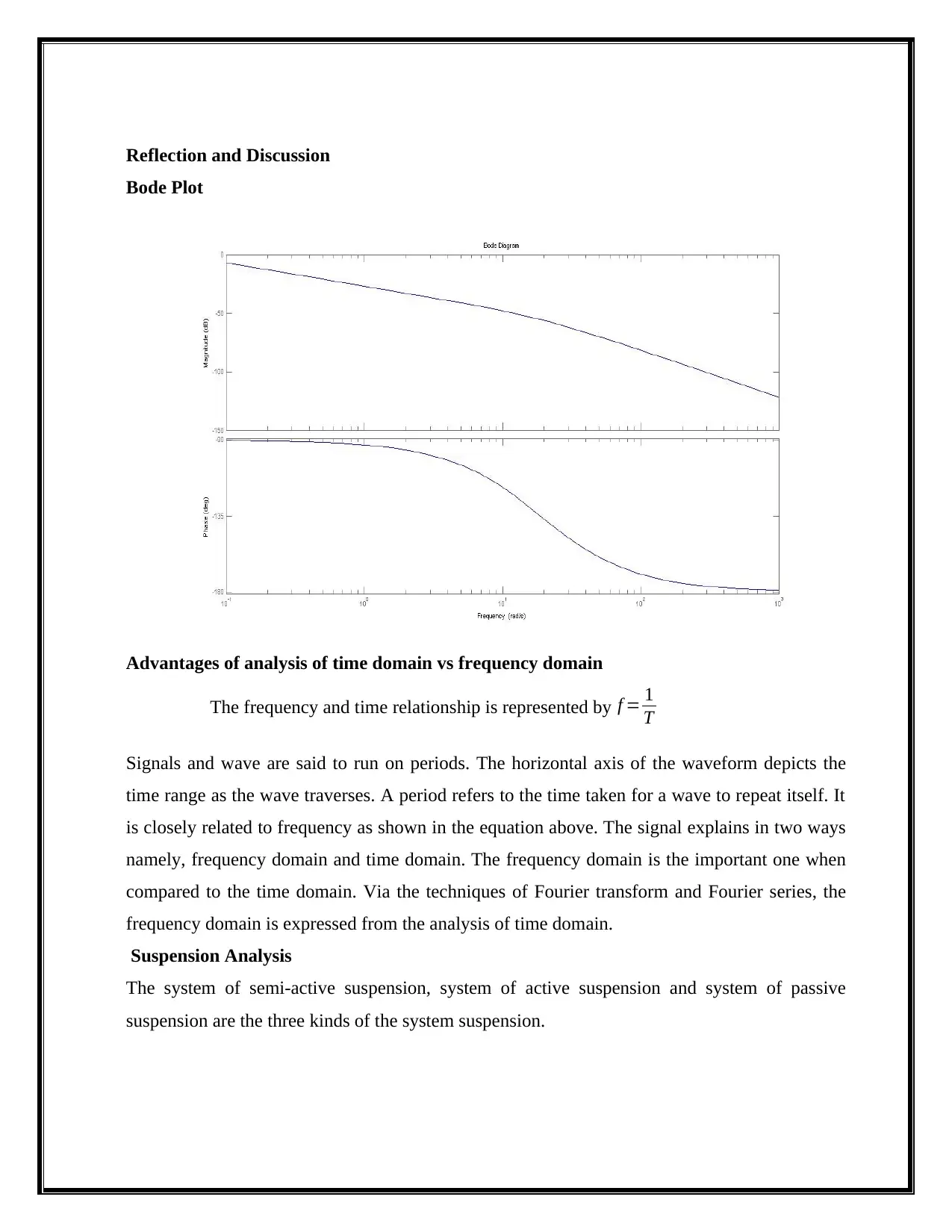
increases and up to the range and suddenly decreased. Compared to bode plot this curve
suddenly decreases. In the magnification graph, the amplitude versus time is plotted in terms of
color representation. The function input represented in green color and the function output
represented by red color. The phase plot shows the value of lag from 0 to pi occurs in each input
frequency. The frequency of input to the output ratio is represents by the r value. The r value is
1 for natural frequency

Reflection and Discussion
Bode Plot
Advantages of analysis of time domain vs frequency domain
The frequency and time relationship is represented by f = 1
T
Signals and wave are said to run on periods. The horizontal axis of the waveform depicts the
time range as the wave traverses. A period refers to the time taken for a wave to repeat itself. It
is closely related to frequency as shown in the equation above. The signal explains in two ways
namely, frequency domain and time domain. The frequency domain is the important one when
compared to the time domain. Via the techniques of Fourier transform and Fourier series, the
frequency domain is expressed from the analysis of time domain.
Suspension Analysis
The system of semi-active suspension, system of active suspension and system of passive
suspension are the three kinds of the system suspension.

11.Conclusion
The system dynamic was simulated via Simulink. With 1DOF, the motorbike mathematical
model was represented by Matlab. For justifying parameters such as seat height, fuel capacity,
wheel mass and bike mass, few assumptions was considered. Via differential degree of freedom
equations domain, the performance of motorbike was done. Found teh operations of matlab via
considered assumptions.
References
DiStefano, J., Stubberud, A. and Williams, I. (2014). Schaum's outline of feedback
and control systems. New York: McGraw-Hill.
Isermann, R. (2014). Digital Control Systems. Berlin: Springer Berlin.
Patrick, D. and Fardo, S. (2009). Industrial process control systems. Atlanta, GA:
Fairmont Press.