Analysis of the Relationship Between Customer Choice and Purchase Decision

The assignment analyzes the relationship between various variables and a customer's choice to purchase chicken using logistic regression. The results show that the display has a significant influence on customer's purchasing decision, with a p-value below 0.05. On the other hand, factors like income (price), feature, and net price do not have a statistically significant impact. The overall accuracy of the model is 57.2%, indicating a moderate level of prediction. The findings suggest that emphasizing display can be an effective strategy for businesses to entice customers.

Econometric

Table of Contents
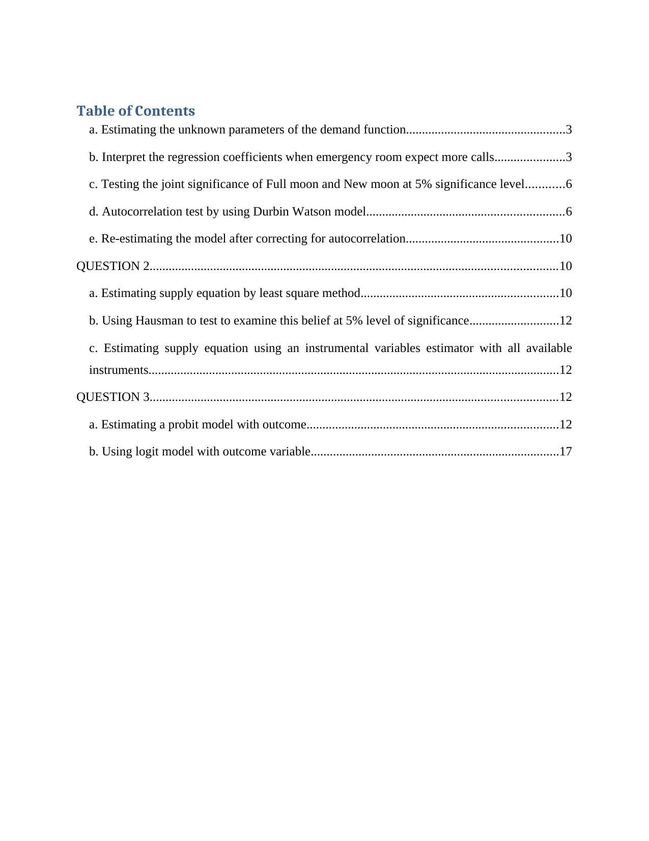
a. Estimating the unknown parameters of the demand function..................................................3
b. Interpret the regression coefficients when emergency room expect more calls......................3
c. Testing the joint significance of Full moon and New moon at 5% significance level............6
d. Autocorrelation test by using Durbin Watson model..............................................................6
e. Re-estimating the model after correcting for autocorrelation................................................10
QUESTION 2................................................................................................................................10
a. Estimating supply equation by least square method..............................................................10
b. Using Hausman to test to examine this belief at 5% level of significance............................12
c. Estimating supply equation using an instrumental variables estimator with all available
instruments.................................................................................................................................12
QUESTION 3................................................................................................................................12
a. Estimating a probit model with outcome...............................................................................12
b. Using logit model with outcome variable..............................................................................17

a. Estimating the unknown parameters of the demand function
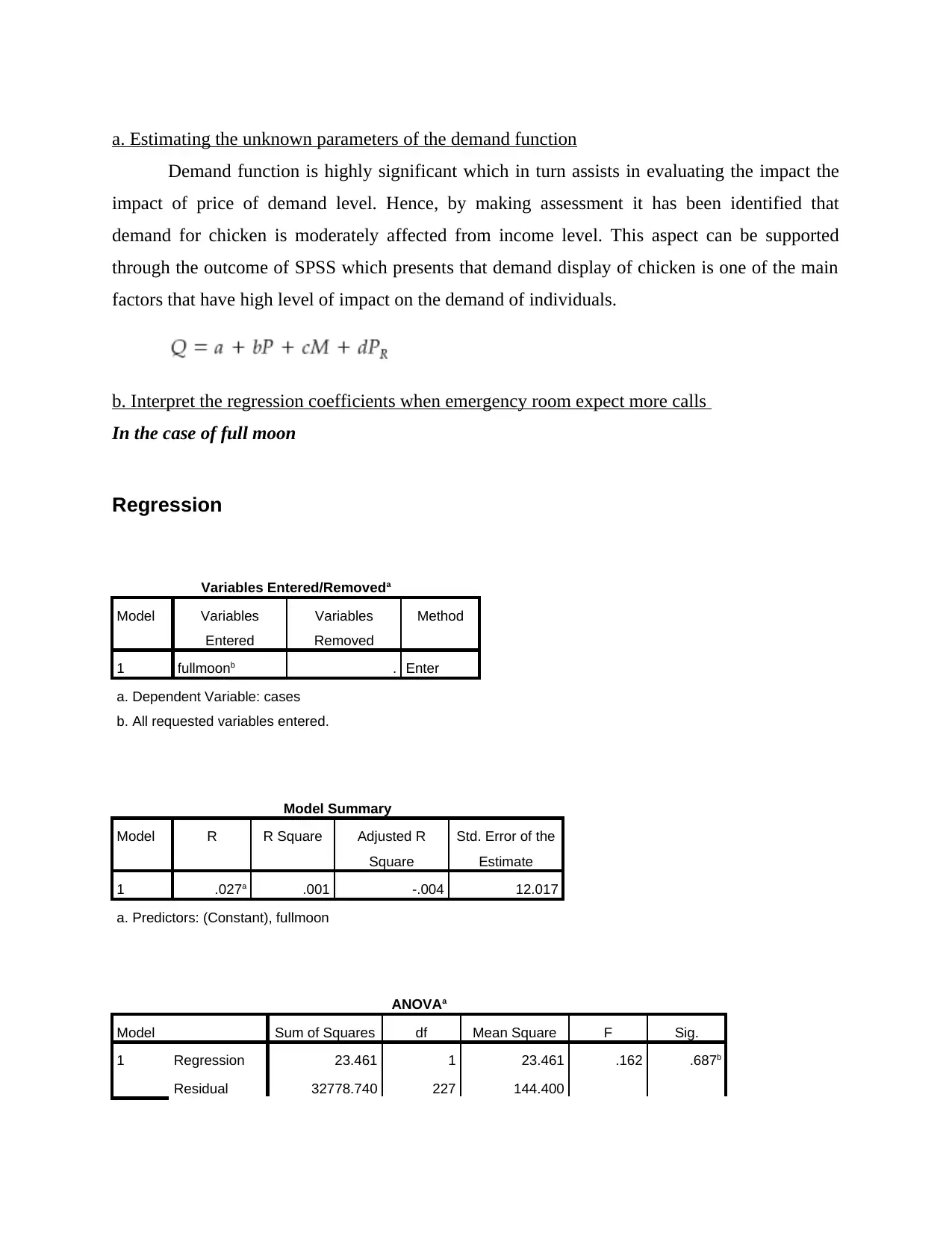
Demand function is highly significant which in turn assists in evaluating the impact the
impact of price of demand level. Hence, by making assessment it has been identified that
demand for chicken is moderately affected from income level. This aspect can be supported
through the outcome of SPSS which presents that demand display of chicken is one of the main
factors that have high level of impact on the demand of individuals.
b. Interpret the regression coefficients when emergency room expect more calls
In the case of full moon
Regression
Variables Entered/Removeda
Model Variables
Entered
Variables
Removed
Method
1 fullmoonb . Enter
a. Dependent Variable: cases
b. All requested variables entered.
Model Summary
Model R R Square Adjusted R
Square
Std. Error of the
Estimate
1 .027a .001 -.004 12.017
a. Predictors: (Constant), fullmoon
ANOVAa
Model Sum of Squares df Mean Square F Sig.
1 Regression 23.461 1 23.461 .162 .687b
Residual 32778.740 227 144.400

Total 32802.201 228
a. Dependent Variable: cases
b. Predictors: (Constant), fullmoon
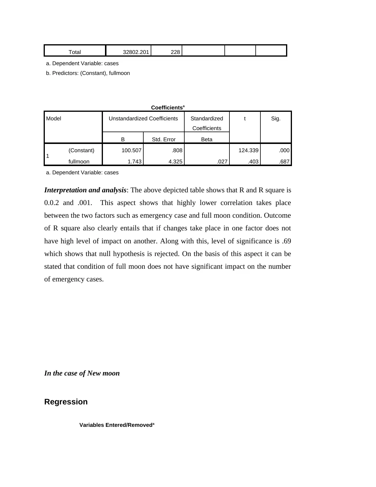
Coefficientsa
Model Unstandardized Coefficients Standardized
Coefficients
t Sig.
B Std. Error Beta
1 (Constant) 100.507 .808 124.339 .000
fullmoon 1.743 4.325 .027 .403 .687
a. Dependent Variable: cases
Interpretation and analysis: The above depicted table shows that R and R square is
0.0.2 and .001. This aspect shows that highly lower correlation takes place
between the two factors such as emergency case and full moon condition. Outcome
of R square also clearly entails that if changes take place in one factor does not
have high level of impact on another. Along with this, level of significance is .69
which shows that null hypothesis is rejected. On the basis of this aspect it can be
stated that condition of full moon does not have significant impact on the number
of emergency cases.
In the case of New moon
Regression
Variables Entered/Removeda

Model Variables
Entered
Variables
Removed
Method
1 newmoonb . Enter
a. Dependent Variable: cases
b. All requested variables entered.
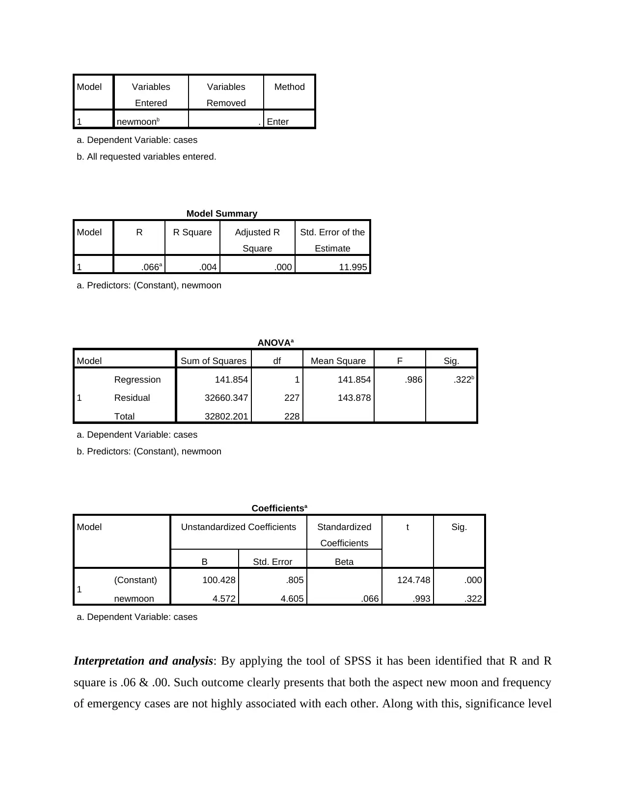
Model Summary
Model R R Square Adjusted R
Square
Std. Error of the
Estimate
1 .066a .004 .000 11.995
a. Predictors: (Constant), newmoon
ANOVAa
Model Sum of Squares df Mean Square F Sig.
1
Regression 141.854 1 141.854 .986 .322b
Residual 32660.347 227 143.878
Total 32802.201 228
a. Dependent Variable: cases
b. Predictors: (Constant), newmoon
Coefficientsa
Model Unstandardized Coefficients Standardized
Coefficients
t Sig.
B Std. Error Beta
1 (Constant) 100.428 .805 124.748 .000
newmoon 4.572 4.605 .066 .993 .322
a. Dependent Variable: cases
Interpretation and analysis: By applying the tool of SPSS it has been identified that R and R
square is .06 & .00. Such outcome clearly presents that both the aspect new moon and frequency
of emergency cases are not highly associated with each other. Along with this, significance level

is greater than standard limit which in turn entails that null hypothesis is accepted and other one
is rejected.
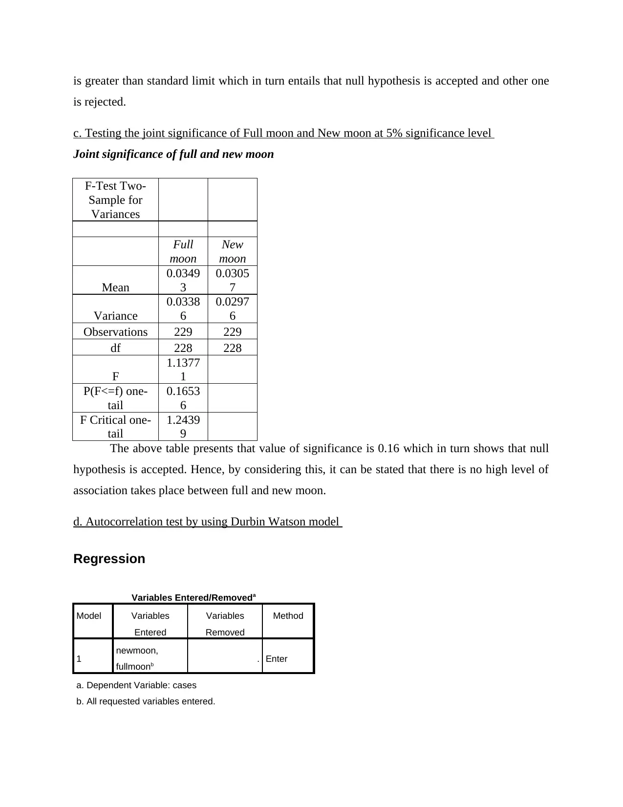
c. Testing the joint significance of Full moon and New moon at 5% significance level
Joint significance of full and new moon
F-Test Two-
Sample for
Variances
Full
moon
New
moon
Mean
0.0349
3
0.0305
7
Variance
0.0338
6
0.0297
6
Observations 229 229
df 228 228
F
1.1377
1
P(F<=f) one-
tail
0.1653
6
F Critical one-
tail
1.2439
9
The above table presents that value of significance is 0.16 which in turn shows that null
hypothesis is accepted. Hence, by considering this, it can be stated that there is no high level of
association takes place between full and new moon.
d. Autocorrelation test by using Durbin Watson model
Regression
Variables Entered/Removeda
Model Variables
Entered
Variables
Removed
Method
1 newmoon,
fullmoonb . Enter
a. Dependent Variable: cases
b. All requested variables entered.

Model Summaryb
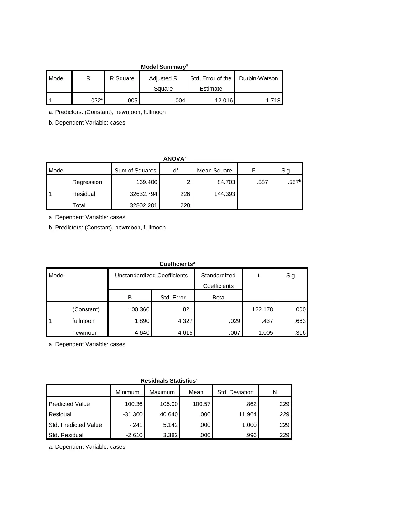
Model R R Square Adjusted R
Square
Std. Error of the
Estimate
Durbin-Watson
1 .072a .005 -.004 12.016 1.718
a. Predictors: (Constant), newmoon, fullmoon
b. Dependent Variable: cases
ANOVAa
Model Sum of Squares df Mean Square F Sig.
1
Regression 169.406 2 84.703 .587 .557b
Residual 32632.794 226 144.393
Total 32802.201 228
a. Dependent Variable: cases
b. Predictors: (Constant), newmoon, fullmoon
Coefficientsa
Model Unstandardized Coefficients Standardized
Coefficients
t Sig.
B Std. Error Beta
1
(Constant) 100.360 .821 122.178 .000
fullmoon 1.890 4.327 .029 .437 .663
newmoon 4.640 4.615 .067 1.005 .316
a. Dependent Variable: cases
Residuals Statisticsa
Minimum Maximum Mean Std. Deviation N
Predicted Value 100.36 105.00 100.57 .862 229
Residual -31.360 40.640 .000 11.964 229
Std. Predicted Value -.241 5.142 .000 1.000 229
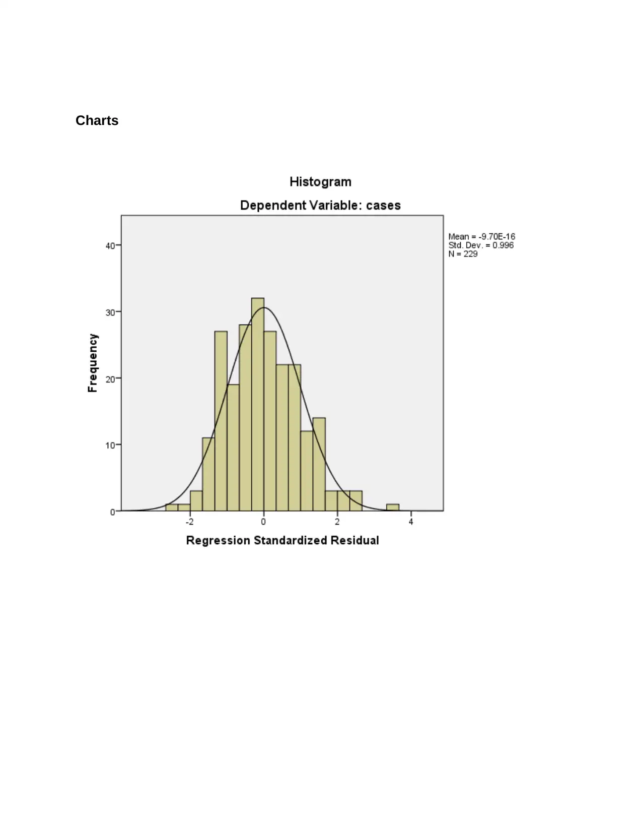
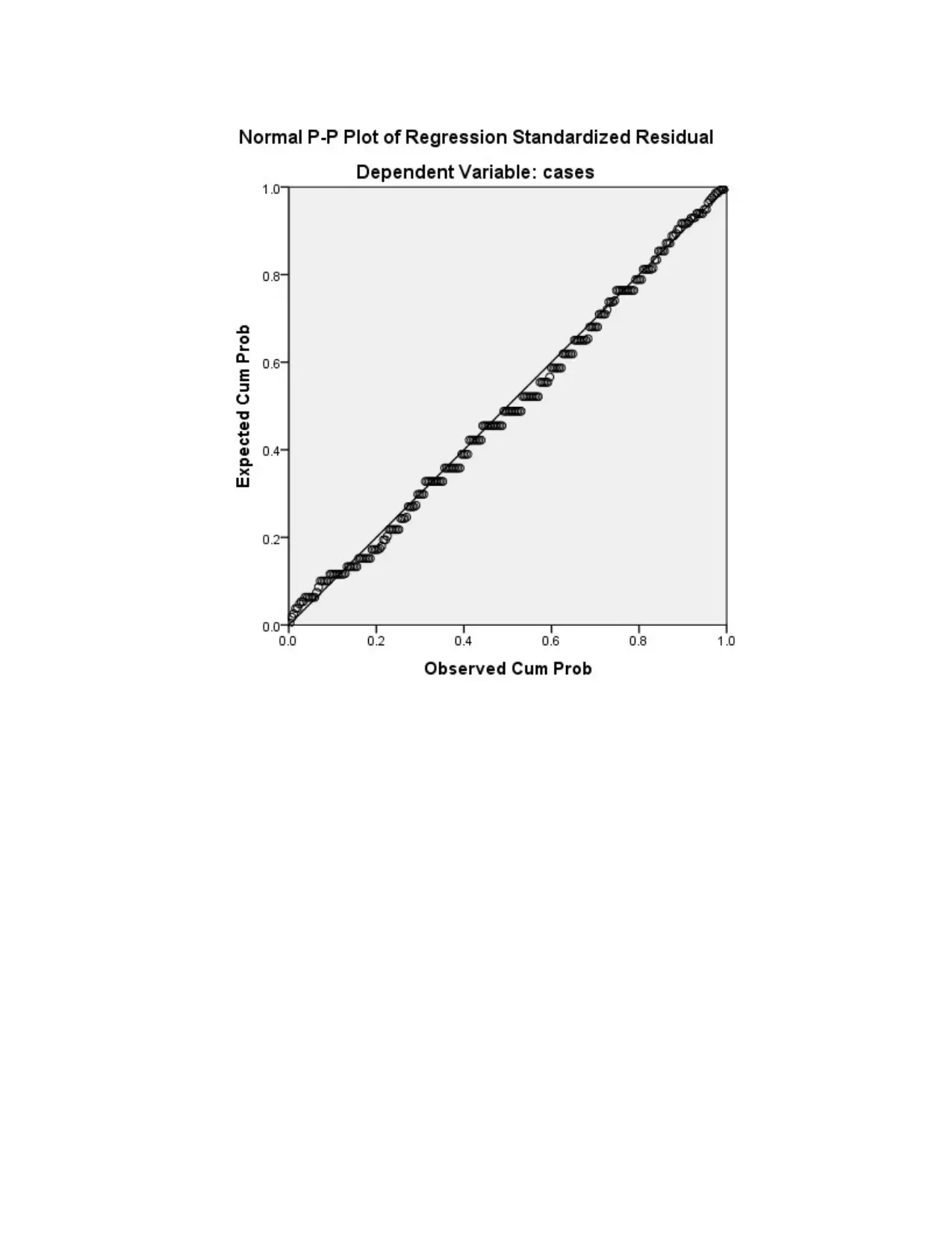
Std. Residual -2.610 3.382 .000 .996 229
a. Dependent Variable: cases

Charts

e. Re-estimating the model after correcting for autocorrelation
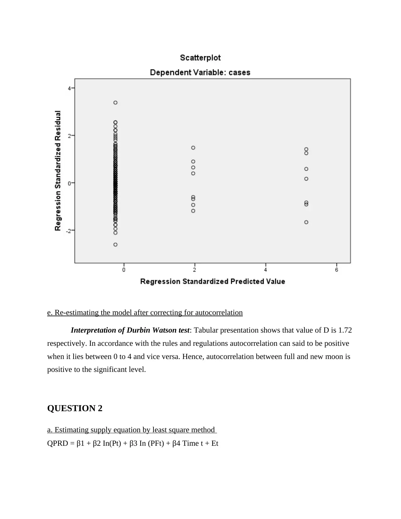
Interpretation of Durbin Watson test: Tabular presentation shows that value of D is 1.72
respectively. In accordance with the rules and regulations autocorrelation can said to be positive
when it lies between 0 to 4 and vice versa. Hence, autocorrelation between full and new moon is
positive to the significant level.
QUESTION 2
a. Estimating supply equation by least square method
QPRD = β1 + β2 In(Pt) + β3 In (PFt) + β4 Time t + Et

Variables Entered/Removeda
Model Variables
Entered
Variables
Removed
Method
1 qb . Enter
a. Dependent Variable: qprod
b. All requested variables entered.
Model Summary
Model R R Square Adjusted R
Square
Std. Error of the
Estimate
1 .979a .959 .958 1146.173
a. Predictors: (Constant), q
ANOVAa
Model Sum of Squares df Mean Square F Sig.
1
Regression 1496691712.44
1 1 1496691712.44
1 1139.284 .000b
Residual 64371929.994 49 1313712.857
Total 1561063642.43
5 50
a. Dependent Variable: qprod
b. Predictors: (Constant), q

Coefficientsa
Model Unstandardized Coefficients Standardized
Coefficients
t Sig.
B Std. Error Beta
1 (Constant) -6479.862 457.034 -14.178 .000
q 469.048 13.896 .979 33.753 .000
a. Dependent Variable: qprod
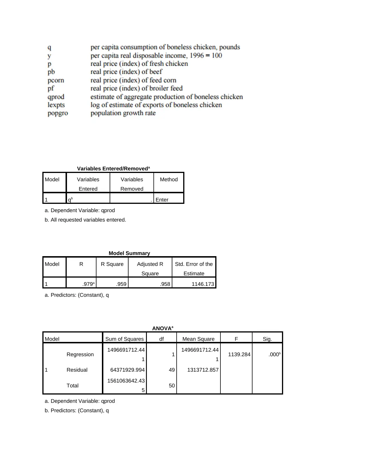
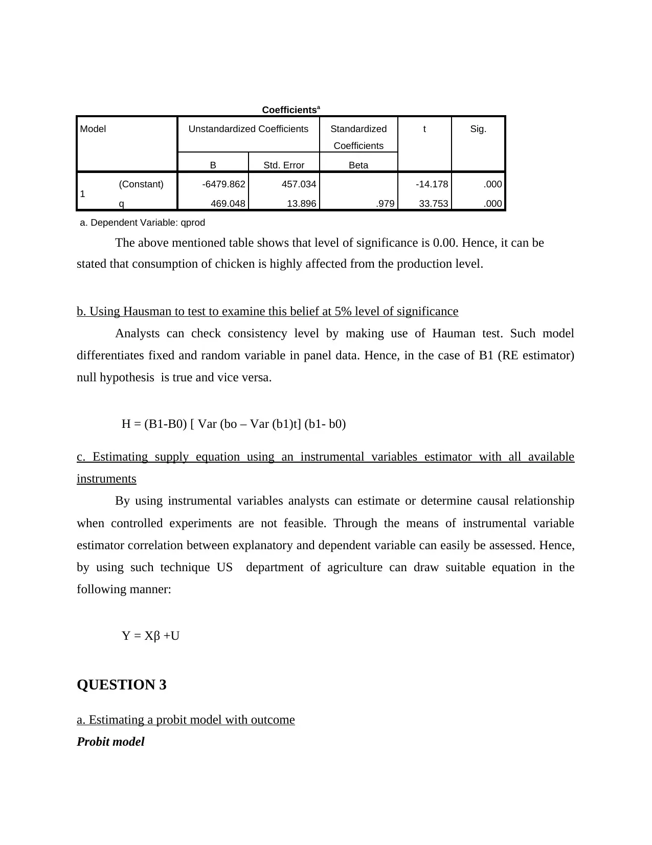
The above mentioned table shows that level of significance is 0.00. Hence, it can be
stated that consumption of chicken is highly affected from the production level.
b. Using Hausman to test to examine this belief at 5% level of significance
Analysts can check consistency level by making use of Hauman test. Such model
differentiates fixed and random variable in panel data. Hence, in the case of B1 (RE estimator)
null hypothesis is true and vice versa.
H = (B1-B0) [ Var (bo – Var (b1)t] (b1- b0)
c. Estimating supply equation using an instrumental variables estimator with all available
instruments
By using instrumental variables analysts can estimate or determine causal relationship
when controlled experiments are not feasible. Through the means of instrumental variable
estimator correlation between explanatory and dependent variable can easily be assessed. Hence,
by using such technique US department of agriculture can draw suitable equation in the
following manner:
Y = Xβ +U
QUESTION 3
a. Estimating a probit model with outcome
Probit model

Descriptive statistics
Descriptive Statistics
N Range Minimum Maximum Mean Std. Deviation Variance
Statistic Statistic Statistic Statistic Statistic Std. Error Statistic Statistic
choice 374 1 0 1 .44 .026 .497 .247
display 374 1 0 1 .07 .014 .264 .069
feature 374 1 0 1 .28 .023 .449 .201
price 374 48 7 55 25.79 .701 13.554 183.699
netprice 374 0 0 1 .67 .006 .110 .012
Valid N (listwise) 374
Frequencies
Statistics
choice
N Valid 374
Missing 0
choice
Frequency Percent Valid Percent Cumulative
Percent
Valid
0 210 56.1 56.1 56.1
1 164 43.9 43.9 100.0
Total 374 100.0 100.0
Frequencies

Statistics
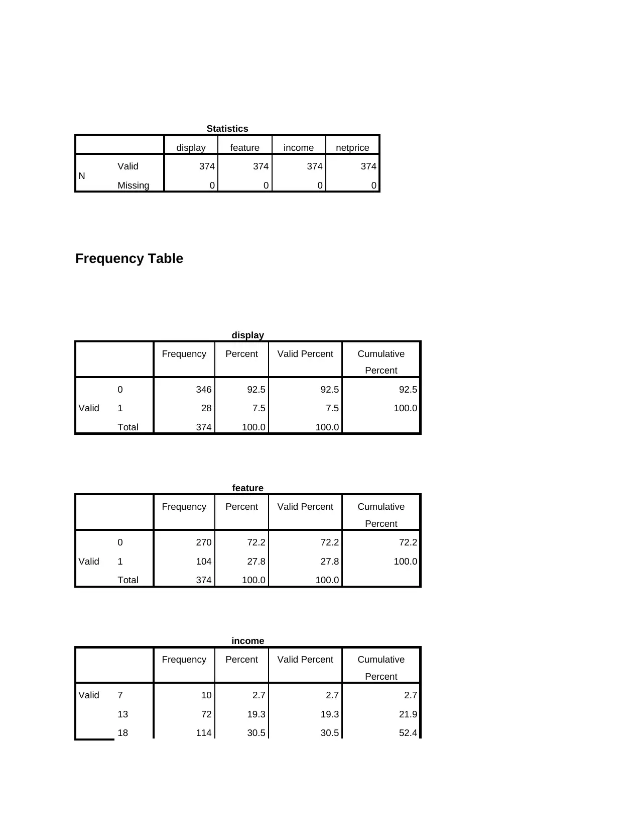
display feature income netprice
N Valid 374 374 374 374
Missing 0 0 0 0
Frequency Table
display
Frequency Percent Valid Percent Cumulative
Percent
Valid
0 346 92.5 92.5 92.5
1 28 7.5 7.5 100.0
Total 374 100.0 100.0
feature
Frequency Percent Valid Percent Cumulative
Percent
Valid
0 270 72.2 72.2 72.2
1 104 27.8 27.8 100.0
Total 374 100.0 100.0
income
Frequency Percent Valid Percent Cumulative
Percent
Valid 7 10 2.7 2.7 2.7
13 72 19.3 19.3 21.9
18 114 30.5 30.5 52.4

23 36 9.6 9.6 62.0
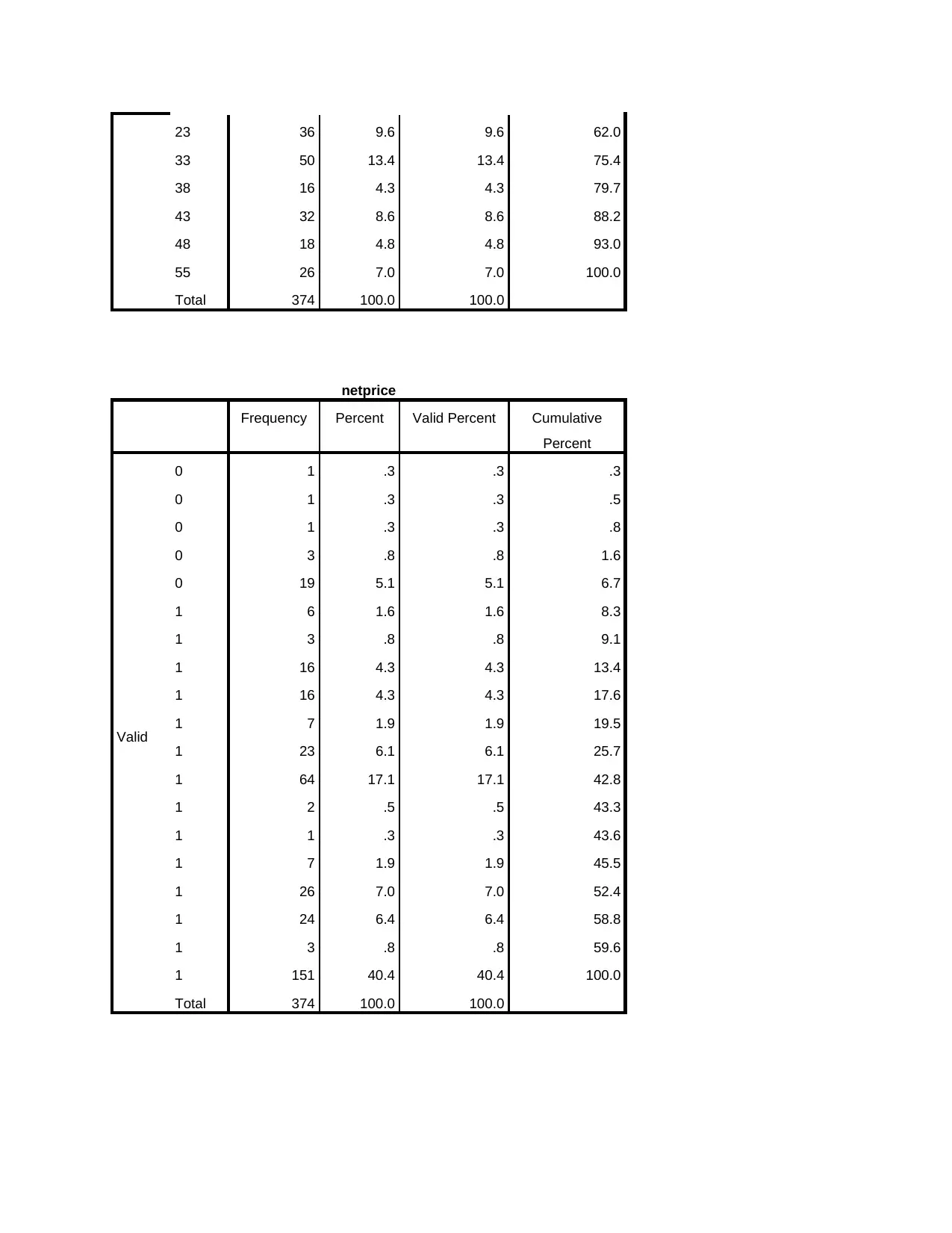
33 50 13.4 13.4 75.4
38 16 4.3 4.3 79.7
43 32 8.6 8.6 88.2
48 18 4.8 4.8 93.0
55 26 7.0 7.0 100.0
Total 374 100.0 100.0
netprice
Frequency Percent Valid Percent Cumulative
Percent
Valid
0 1 .3 .3 .3
0 1 .3 .3 .5
0 1 .3 .3 .8
0 3 .8 .8 1.6
0 19 5.1 5.1 6.7
1 6 1.6 1.6 8.3
1 3 .8 .8 9.1
1 16 4.3 4.3 13.4
1 16 4.3 4.3 17.6
1 7 1.9 1.9 19.5
1 23 6.1 6.1 25.7
1 64 17.1 17.1 42.8
1 2 .5 .5 43.3
1 1 .3 .3 43.6
1 7 1.9 1.9 45.5
1 26 7.0 7.0 52.4
1 24 6.4 6.4 58.8
1 3 .8 .8 59.6
1 151 40.4 40.4 100.0
Total 374 100.0 100.0

PLUM - Ordinal Regression
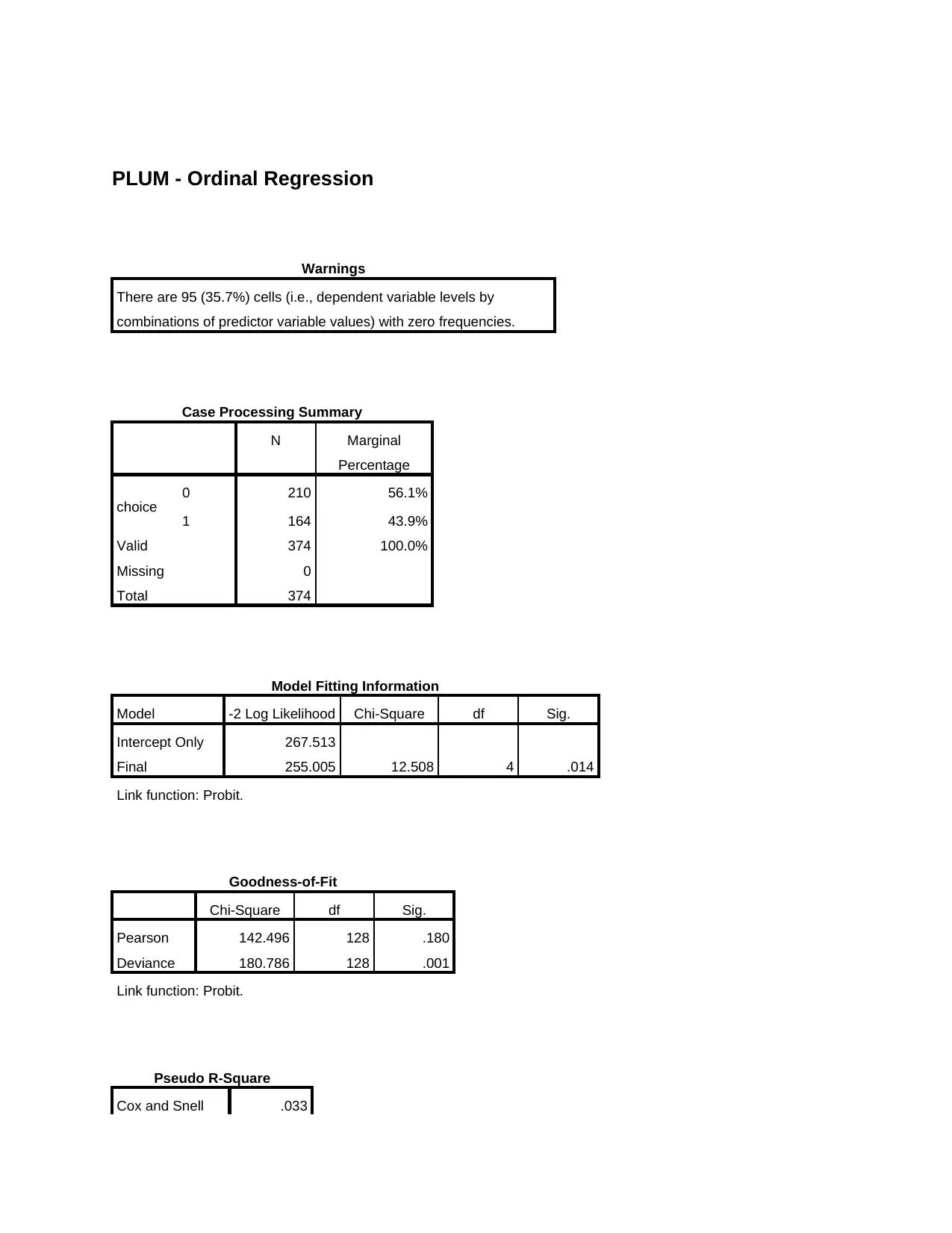
Warnings
There are 95 (35.7%) cells (i.e., dependent variable levels by
combinations of predictor variable values) with zero frequencies.
Case Processing Summary
N Marginal
Percentage
choice 0 210 56.1%
1 164 43.9%
Valid 374 100.0%
Missing 0
Total 374
Model Fitting Information
Model -2 Log Likelihood Chi-Square df Sig.
Intercept Only 267.513
Final 255.005 12.508 4 .014
Link function: Probit.
Goodness-of-Fit
Chi-Square df Sig.
Pearson 142.496 128 .180
Deviance 180.786 128 .001
Link function: Probit.
Pseudo R-Square
Cox and Snell .033

Nagelkerke .044
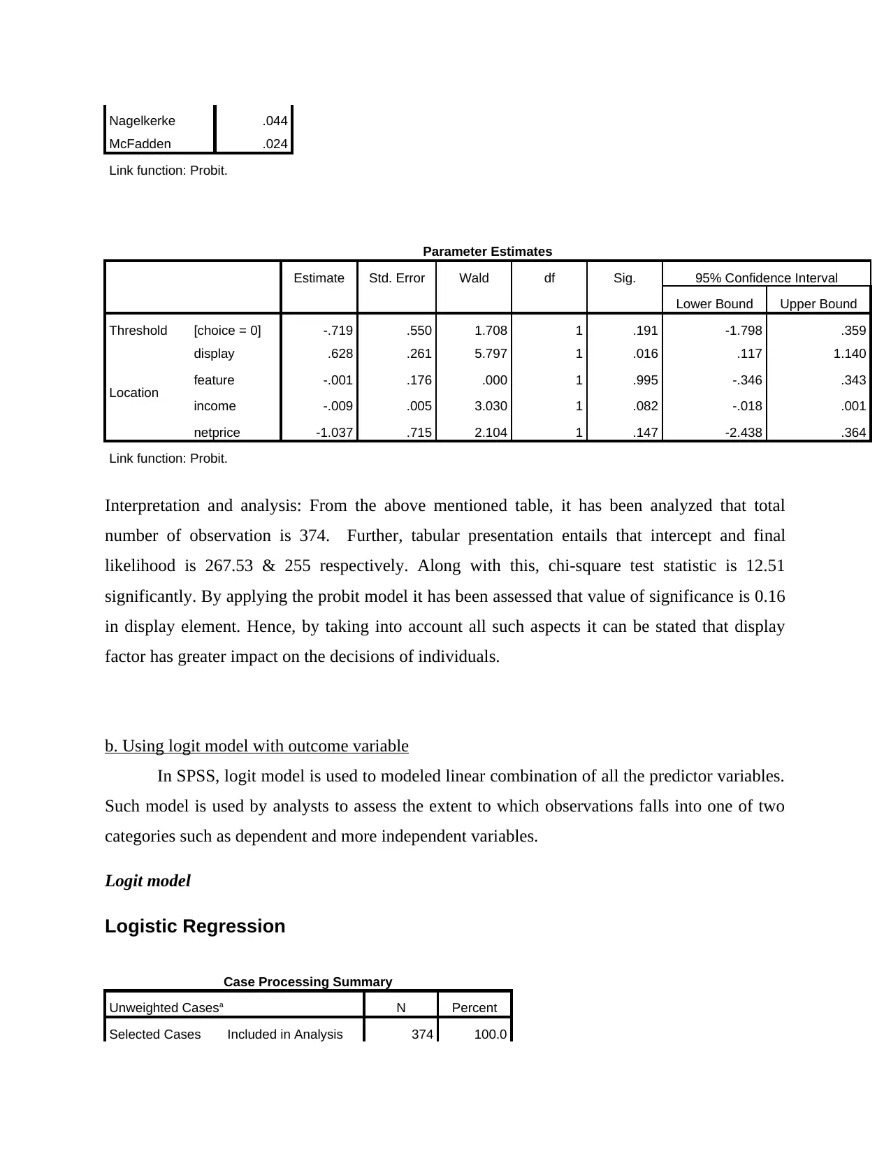
McFadden .024
Link function: Probit.
Parameter Estimates
Estimate Std. Error Wald df Sig. 95% Confidence Interval
Lower Bound Upper Bound
Threshold [choice = 0] -.719 .550 1.708 1 .191 -1.798 .359
Location
display .628 .261 5.797 1 .016 .117 1.140
feature -.001 .176 .000 1 .995 -.346 .343
income -.009 .005 3.030 1 .082 -.018 .001
netprice -1.037 .715 2.104 1 .147 -2.438 .364
Link function: Probit.
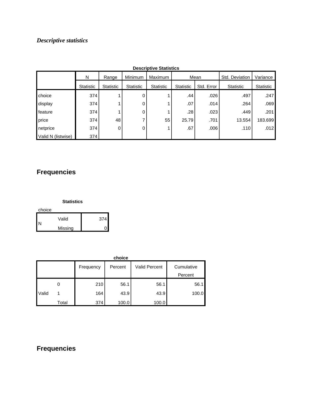
Interpretation and analysis: From the above mentioned table, it has been analyzed that total
number of observation is 374. Further, tabular presentation entails that intercept and final
likelihood is 267.53 & 255 respectively. Along with this, chi-square test statistic is 12.51
significantly. By applying the probit model it has been assessed that value of significance is 0.16
in display element. Hence, by taking into account all such aspects it can be stated that display
factor has greater impact on the decisions of individuals.
b. Using logit model with outcome variable
In SPSS, logit model is used to modeled linear combination of all the predictor variables.
Such model is used by analysts to assess the extent to which observations falls into one of two
categories such as dependent and more independent variables.
Logit model
Logistic Regression
Case Processing Summary
Unweighted Casesa N Percent
Selected Cases Included in Analysis 374 100.0

Missing Cases 0 .0
Total 374 100.0
Unselected Cases 0 .0
Total 374 100.0
a. If weight is in effect, see classification table for the total number of
cases.
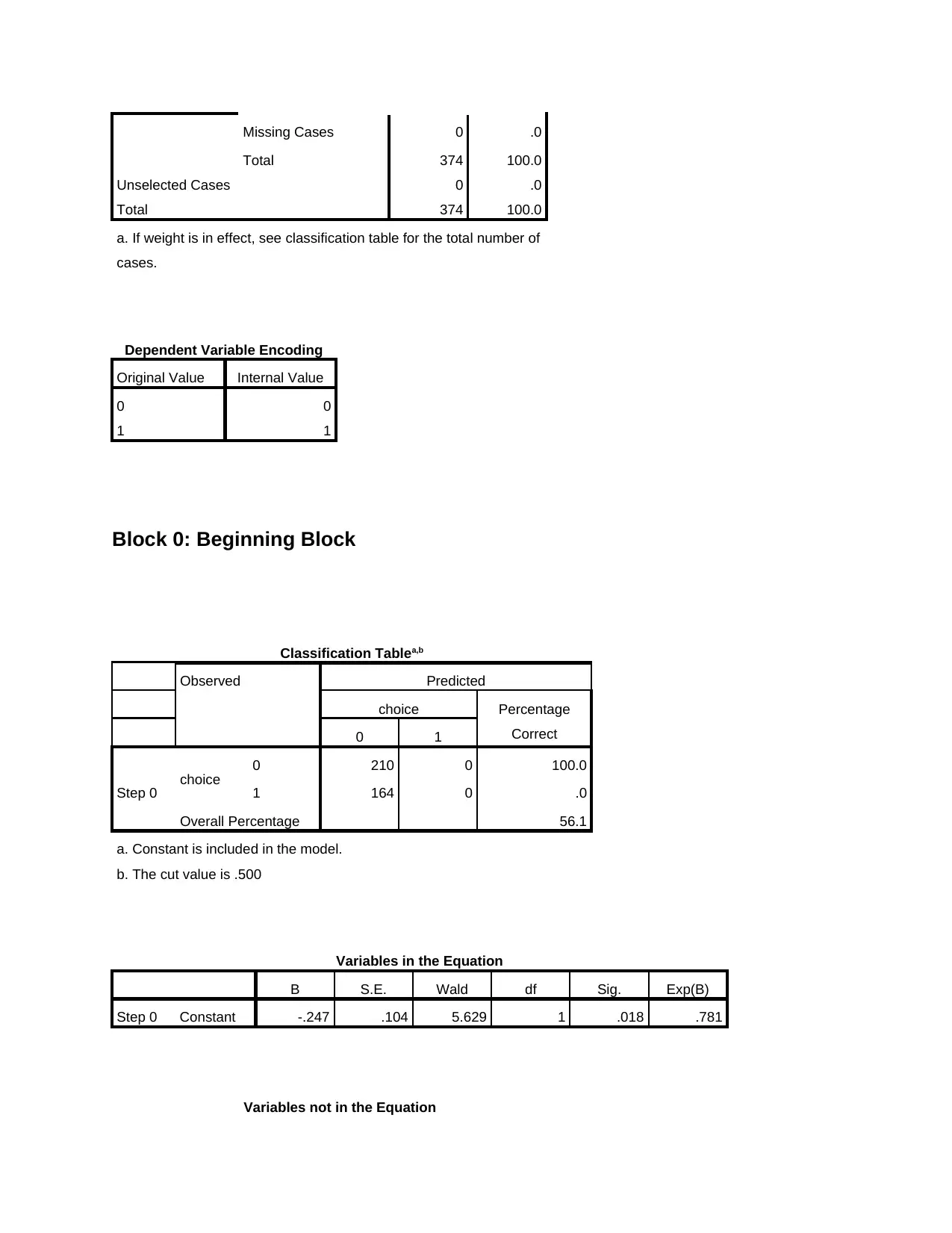
Dependent Variable Encoding
Original Value Internal Value
0 0
1 1
Block 0: Beginning Block
Classification Tablea,b
Observed Predicted
choice Percentage
Correct0 1
Step 0 choice 0 210 0 100.0
1 164 0 .0
Overall Percentage 56.1
a. Constant is included in the model.
b. The cut value is .500
Variables in the Equation
B S.E. Wald df Sig. Exp(B)
Step 0 Constant -.247 .104 5.629 1 .018 .781
Variables not in the Equation

Score df Sig.
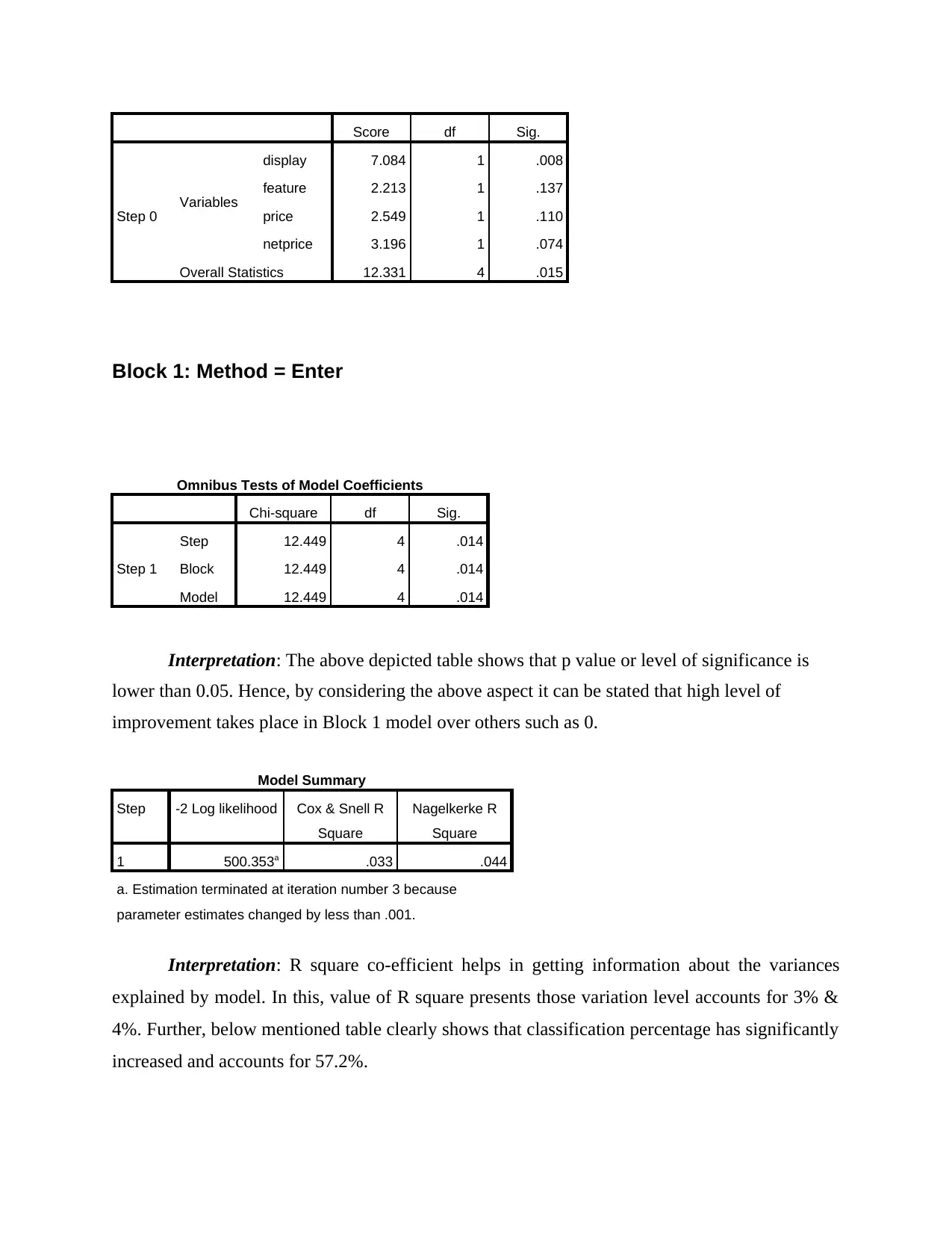
Step 0 Variables
display 7.084 1 .008
feature 2.213 1 .137
price 2.549 1 .110
netprice 3.196 1 .074
Overall Statistics 12.331 4 .015
Block 1: Method = Enter
Omnibus Tests of Model Coefficients
Chi-square df Sig.
Step 1
Step 12.449 4 .014
Block 12.449 4 .014
Model 12.449 4 .014
Interpretation: The above depicted table shows that p value or level of significance is
lower than 0.05. Hence, by considering the above aspect it can be stated that high level of
improvement takes place in Block 1 model over others such as 0.
Model Summary
Step -2 Log likelihood Cox & Snell R
Square
Nagelkerke R
Square
1 500.353a .033 .044
a. Estimation terminated at iteration number 3 because
parameter estimates changed by less than .001.
Interpretation: R square co-efficient helps in getting information about the variances
explained by model. In this, value of R square presents those variation level accounts for 3% &
4%. Further, below mentioned table clearly shows that classification percentage has significantly
increased and accounts for 57.2%.

Classification Tablea
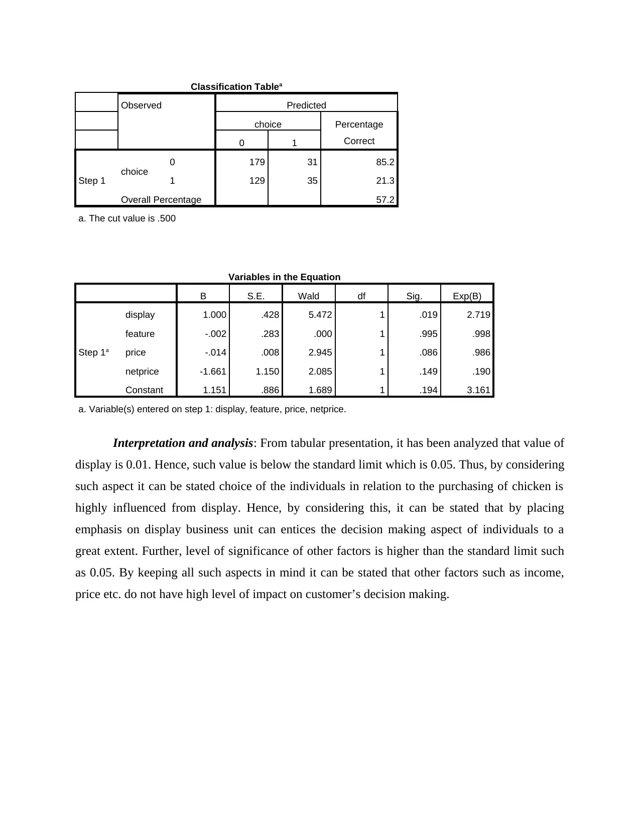
Observed Predicted
choice Percentage
Correct0 1
Step 1 choice 0 179 31 85.2
1 129 35 21.3
Overall Percentage 57.2
a. The cut value is .500
Variables in the Equation
B S.E. Wald df Sig. Exp(B)
Step 1a
display 1.000 .428 5.472 1 .019 2.719
feature -.002 .283 .000 1 .995 .998
price -.014 .008 2.945 1 .086 .986
netprice -1.661 1.150 2.085 1 .149 .190
Constant 1.151 .886 1.689 1 .194 3.161
a. Variable(s) entered on step 1: display, feature, price, netprice.
Interpretation and analysis: From tabular presentation, it has been analyzed that value of
display is 0.01. Hence, such value is below the standard limit which is 0.05. Thus, by considering
such aspect it can be stated choice of the individuals in relation to the purchasing of chicken is
highly influenced from display. Hence, by considering this, it can be stated that by placing
emphasis on display business unit can entices the decision making aspect of individuals to a
great extent. Further, level of significance of other factors is higher than the standard limit such
as 0.05. By keeping all such aspects in mind it can be stated that other factors such as income,
price etc. do not have high level of impact on customer’s decision making.