Econometrics - Analysis of MARKET2022, OECDINCOME2022 and SHAREPRICE2022

This article provides an analysis of MARKET2022, OECDINCOME2022 and SHAREPRICE2022 using econometrics. It includes descriptive statistics, correlations, model summary, ANOVA, and coefficients. The article also includes interpretation and predictions based on the results.

Econometrics

Contents
TASK...............................................................................................................................................3
4. File related is MARKET2022..................................................................................................3
5. OECDINCOME2022 is related with the income and expenditure of the people....................4
6. SHAREPRICE2022 is related with the variable of ShareA and ShareB.................................6
REFERENCES................................................................................................................................8

TASK
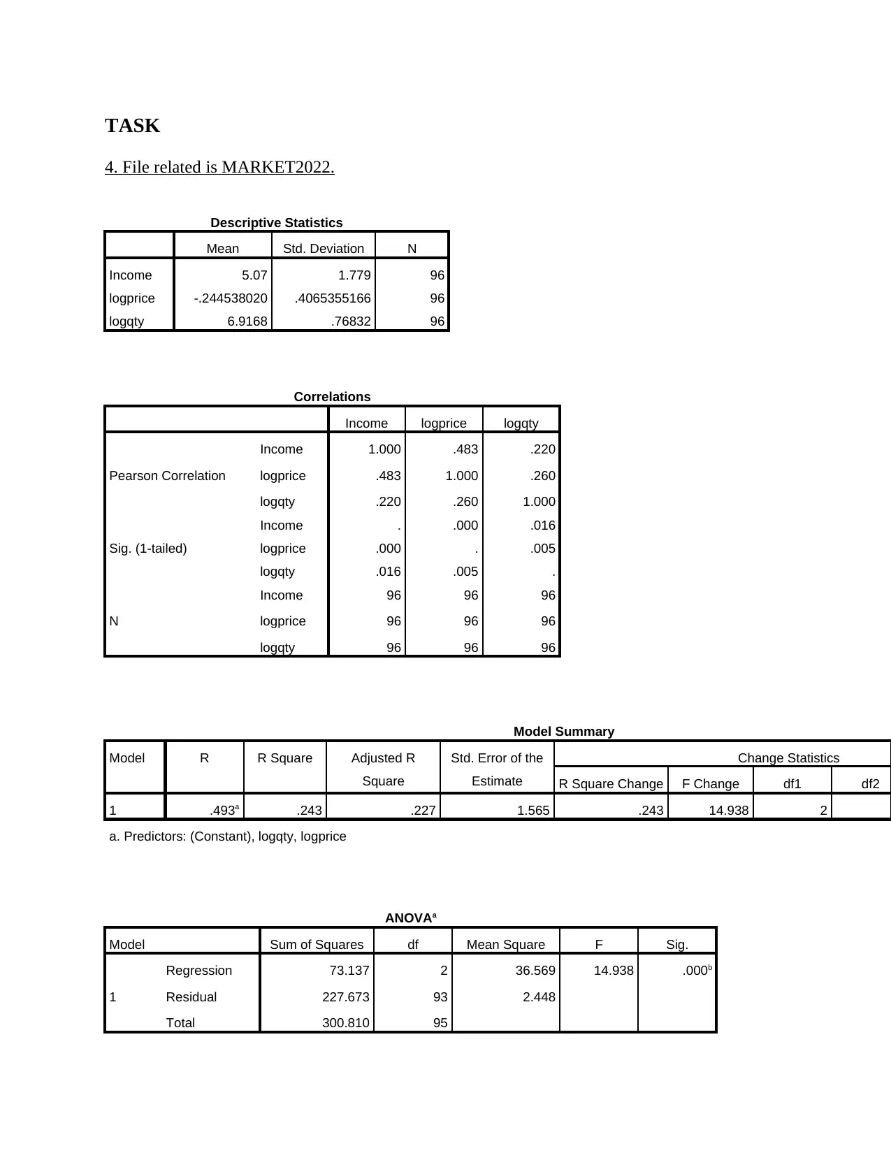
4. File related is MARKET2022.
Descriptive Statistics
Mean Std. Deviation N
Income 5.07 1.779 96
logprice -.244538020 .4065355166 96
logqty 6.9168 .76832 96
Correlations
Income logprice logqty
Pearson Correlation
Income 1.000 .483 .220
logprice .483 1.000 .260
logqty .220 .260 1.000
Sig. (1-tailed)
Income . .000 .016
logprice .000 . .005
logqty .016 .005 .
N
Income 96 96 96
logprice 96 96 96
logqty 96 96 96
Model Summary
Model R R Square Adjusted R
Square
Std. Error of the
Estimate
Change Statistics
R Square Change F Change df1 df2
1 .493a .243 .227 1.565 .243 14.938 2 9
a. Predictors: (Constant), logqty, logprice
ANOVAa
Model Sum of Squares df Mean Square F Sig.
1
Regression 73.137 2 36.569 14.938 .000b
Residual 227.673 93 2.448
Total 300.810 95

a. Dependent Variable: Income
b. Predictors: (Constant), logqty, logprice
Coefficientsa
Model Unstandardized Coefficients Standardized
Coefficients
t Sig.
B Std. Error Beta
1
(Constant) 3.938 1.534 2.567 .012
logprice 2.000 .409 .457 4.891 .000
logqty .234 .216 .101 1.082 .282
a. Dependent Variable: Income
Interpretation: From the above run test it can be interpreted and predicted that the supply
equation which is denoted as logqty and demand equation which is quoted as logprices show that
there is a significant relationship existing between both variables. The two equation system takes
in account logprices and logqty which indicates the quantity being supplied and demand being
generated in relation with the prices. Yes, the supply equation is being identified which is logqty
indicating how much the quantity is being demanded and served by the consumers and facilitated
by company. It is observed that there is a moderate impact assessed between two equations
which also helps in predicting values in relation to another element. The supply equation is also
identified as logqty which would help to know the quantity of goods being supplied. There is
always a related change observed when the price of product changes which also would impact
the quantity being supplied in the market. Such impact can be examined with the help of
regression equation explaining the impact of price change on quantity being demanded and
supplied (Pauwels, 2018).
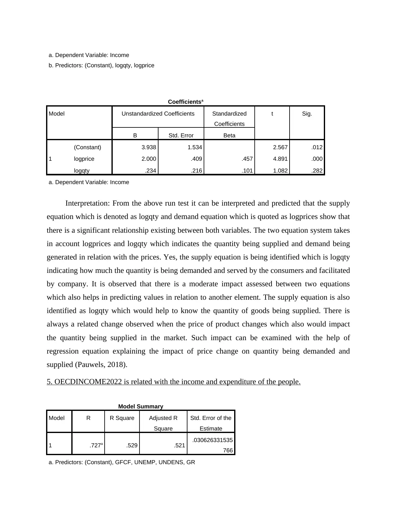
5. OECDINCOME2022 is related with the income and expenditure of the people.
Model Summary
Model R R Square Adjusted R
Square
Std. Error of the
Estimate
1 .727a .529 .521 .030626331535
766
a. Predictors: (Constant), GFCF, UNEMP, UNDENS, GR

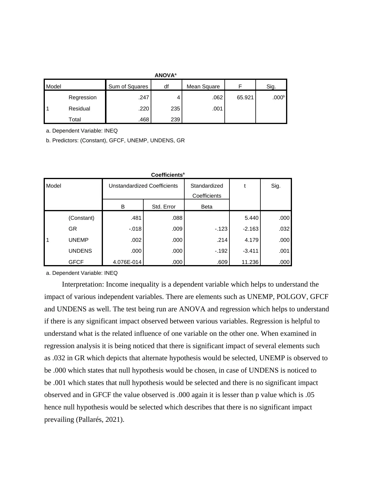
ANOVAa
Model Sum of Squares df Mean Square F Sig.
1
Regression .247 4 .062 65.921 .000b
Residual .220 235 .001
Total .468 239
a. Dependent Variable: INEQ
b. Predictors: (Constant), GFCF, UNEMP, UNDENS, GR
Coefficientsa
Model Unstandardized Coefficients Standardized
Coefficients
t Sig.
B Std. Error Beta
1
(Constant) .481 .088 5.440 .000
GR -.018 .009 -.123 -2.163 .032
UNEMP .002 .000 .214 4.179 .000
UNDENS .000 .000 -.192 -3.411 .001
GFCF 4.076E-014 .000 .609 11.236 .000
a. Dependent Variable: INEQ
Interpretation: Income inequality is a dependent variable which helps to understand the
impact of various independent variables. There are elements such as UNEMP, POLGOV, GFCF
and UNDENS as well. The test being run are ANOVA and regression which helps to understand
if there is any significant impact observed between various variables. Regression is helpful to
understand what is the related influence of one variable on the other one. When examined in
regression analysis it is being noticed that there is significant impact of several elements such
as .032 in GR which depicts that alternate hypothesis would be selected, UNEMP is observed to
be .000 which states that null hypothesis would be chosen, in case of UNDENS is noticed to
be .001 which states that null hypothesis would be selected and there is no significant impact
observed and in GFCF the value observed is .000 again it is lesser than p value which is .05
hence null hypothesis would be selected which describes that there is no significant impact
prevailing (Pallarés, 2021).

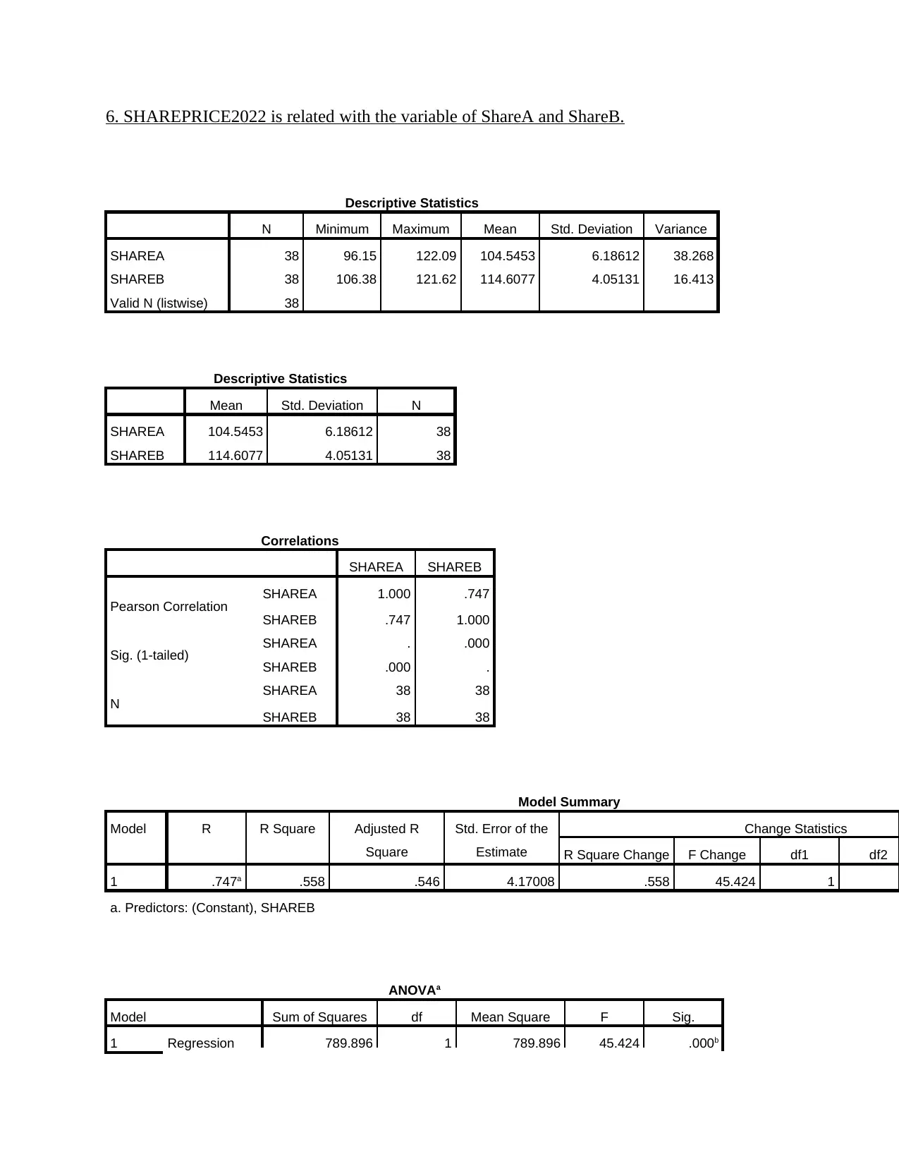
6. SHAREPRICE2022 is related with the variable of ShareA and ShareB.
Descriptive Statistics
N Minimum Maximum Mean Std. Deviation Variance
SHAREA 38 96.15 122.09 104.5453 6.18612 38.268
SHAREB 38 106.38 121.62 114.6077 4.05131 16.413
Valid N (listwise) 38
Descriptive Statistics
Mean Std. Deviation N
SHAREA 104.5453 6.18612 38
SHAREB 114.6077 4.05131 38
Correlations
SHAREA SHAREB
Pearson Correlation SHAREA 1.000 .747
SHAREB .747 1.000
Sig. (1-tailed) SHAREA . .000
SHAREB .000 .
N SHAREA 38 38
SHAREB 38 38
Model Summary
Model R R Square Adjusted R
Square
Std. Error of the
Estimate
Change Statistics
R Square Change F Change df1 df2
1 .747a .558 .546 4.17008 .558 45.424 1 3
a. Predictors: (Constant), SHAREB
ANOVAa
Model Sum of Squares df Mean Square F Sig.
1 Regression 789.896 1 789.896 45.424 .000b

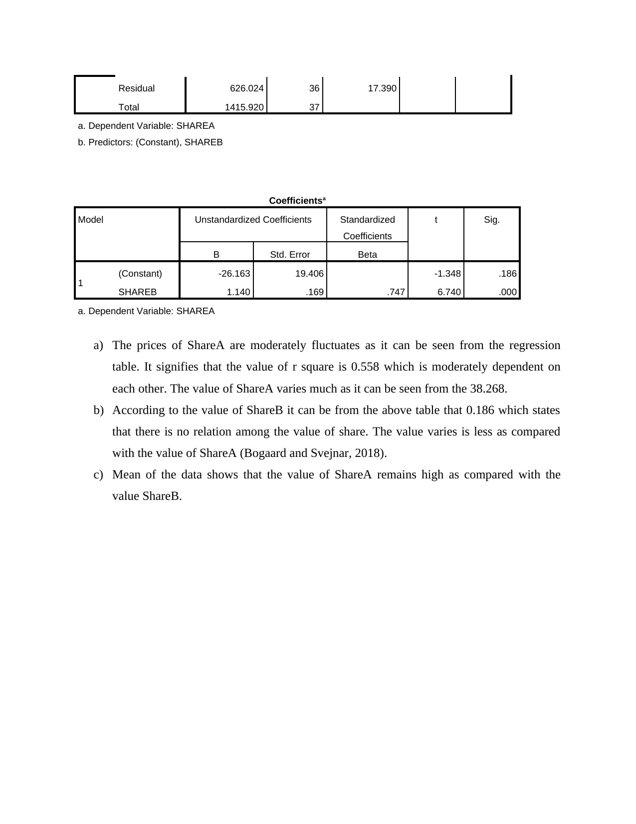
Residual 626.024 36 17.390
Total 1415.920 37
a. Dependent Variable: SHAREA
b. Predictors: (Constant), SHAREB
Coefficientsa
Model Unstandardized Coefficients Standardized
Coefficients
t Sig.
B Std. Error Beta
1 (Constant) -26.163 19.406 -1.348 .186
SHAREB 1.140 .169 .747 6.740 .000
a. Dependent Variable: SHAREA
a) The prices of ShareA are moderately fluctuates as it can be seen from the regression
table. It signifies that the value of r square is 0.558 which is moderately dependent on
each other. The value of ShareA varies much as it can be seen from the 38.268.
b) According to the value of ShareB it can be from the above table that 0.186 which states
that there is no relation among the value of share. The value varies is less as compared
with the value of ShareA (Bogaard and Svejnar, 2018).
c) Mean of the data shows that the value of ShareA remains high as compared with the
value ShareB.

REFERENCES
Books and Journals
Bogaard, H. and Svejnar, J., 2018. Incentive pay and performance: Insider econometrics in a
multi-unit firm. Labour Economics. 54. pp.100-115.
Koopman, S.J. and et.al., 2019. A., “Dynamic Discrete Copula Models for High Frequency Stock
Price Changes”, Journal of Applied Econometrics, forthcoming.
Nguyen, H.P., 2018. Why Hammerstein-Type Block Models Are so Efficient: Case Study of
Financial Econometrics. Beyond Traditional Probabilistic Methods in Economics. 809.
p.129.
Pallarés, N., 2021. Three Essays in Applied Econometrics.
Pauwels, K., 2018. How time series econometrics helped Inofec quantify online and offline
funnel progression and reallocate marketing budgets for higher profits. In Handbook of
Marketing Analytics. Edward Elgar Publishing.