Econometrics Assignment - Linear Regression, Interactions, Heteroscedasticity, OLS Coefficients

This assignment covers topics such as linear regression, interactions, heteroscedasticity, OLS coefficients, and more. It includes interpretations of coefficients, F-statistics, Chow tests, and error variance.

Running head: ECONOMETRICS ASSIGNMENT
Econometrics Assignment
Name
Course Number
Date
Faculty Name

ECONOMETRICS ASSIGNMENT 2
Econometrics Assignment
Question 1: Linear Regression
1. Private and non-private colleges
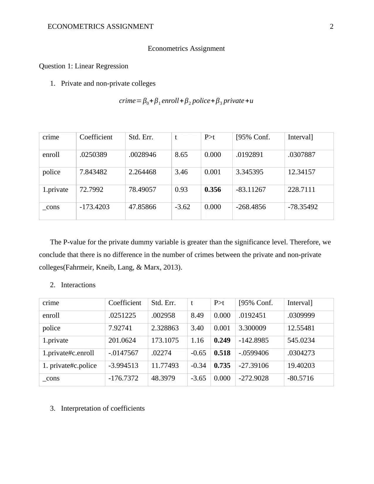
crime= β0 + β1 enroll+ β2 police+ β3 private +u
crime Coefficient Std. Err. t P>t [95% Conf. Interval]
enroll .0250389 .0028946 8.65 0.000 .0192891 .0307887
police 7.843482 2.264468 3.46 0.001 3.345395 12.34157
1.private 72.7992 78.49057 0.93 0.356 -83.11267 228.7111
_cons -173.4203 47.85866 -3.62 0.000 -268.4856 -78.35492
The P-value for the private dummy variable is greater than the significance level. Therefore, we
conclude that there is no difference in the number of crimes between the private and non-private
colleges(Fahrmeir, Kneib, Lang, & Marx, 2013).
2. Interactions
crime Coefficient Std. Err. t P>t [95% Conf. Interval]
enroll .0251225 .002958 8.49 0.000 .0192451 .0309999
police 7.92741 2.328863 3.40 0.001 3.300009 12.55481
1.private 201.0624 173.1075 1.16 0.249 -142.8985 545.0234
1.private#c.enroll -.0147567 .02274 -0.65 0.518 -.0599406 .0304273
1. private#c.police -3.994513 11.77493 -0.34 0.735 -27.39106 19.40203
_cons -176.7372 48.3979 -3.65 0.000 -272.9028 -80.5716
3. Interpretation of coefficients

ECONOMETRICS ASSIGNMENT 3
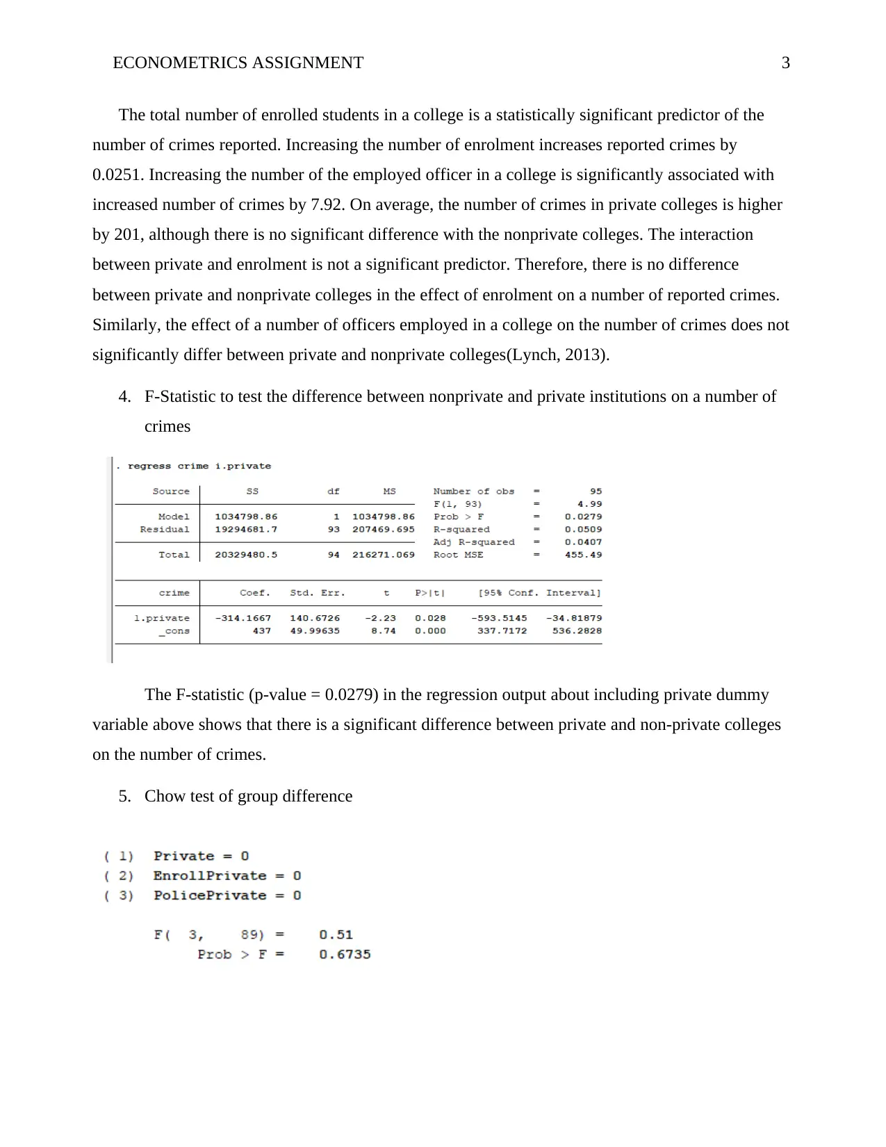
The total number of enrolled students in a college is a statistically significant predictor of the
number of crimes reported. Increasing the number of enrolment increases reported crimes by
0.0251. Increasing the number of the employed officer in a college is significantly associated with
increased number of crimes by 7.92. On average, the number of crimes in private colleges is higher
by 201, although there is no significant difference with the nonprivate colleges. The interaction
between private and enrolment is not a significant predictor. Therefore, there is no difference
between private and nonprivate colleges in the effect of enrolment on a number of reported crimes.
Similarly, the effect of a number of officers employed in a college on the number of crimes does not
significantly differ between private and nonprivate colleges(Lynch, 2013).
4. F-Statistic to test the difference between nonprivate and private institutions on a number of
crimes
The F-statistic (p-value = 0.0279) in the regression output about including private dummy
variable above shows that there is a significant difference between private and non-private colleges
on the number of crimes.
5. Chow test of group difference

ECONOMETRICS ASSIGNMENT 4
Using the Chow test, we can conclude that there is no difference in intercepts and slopes between
privates and non-privates colleges.
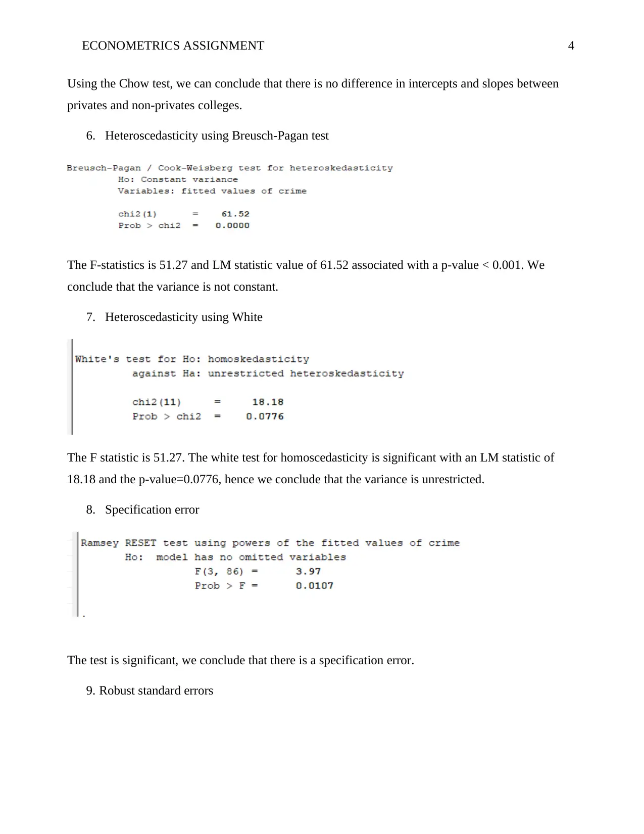
6. Heteroscedasticity using Breusch-Pagan test
The F-statistics is 51.27 and LM statistic value of 61.52 associated with a p-value < 0.001. We
conclude that the variance is not constant.
7. Heteroscedasticity using White
The F statistic is 51.27. The white test for homoscedasticity is significant with an LM statistic of
18.18 and the p-value=0.0776, hence we conclude that the variance is unrestricted.
8. Specification error
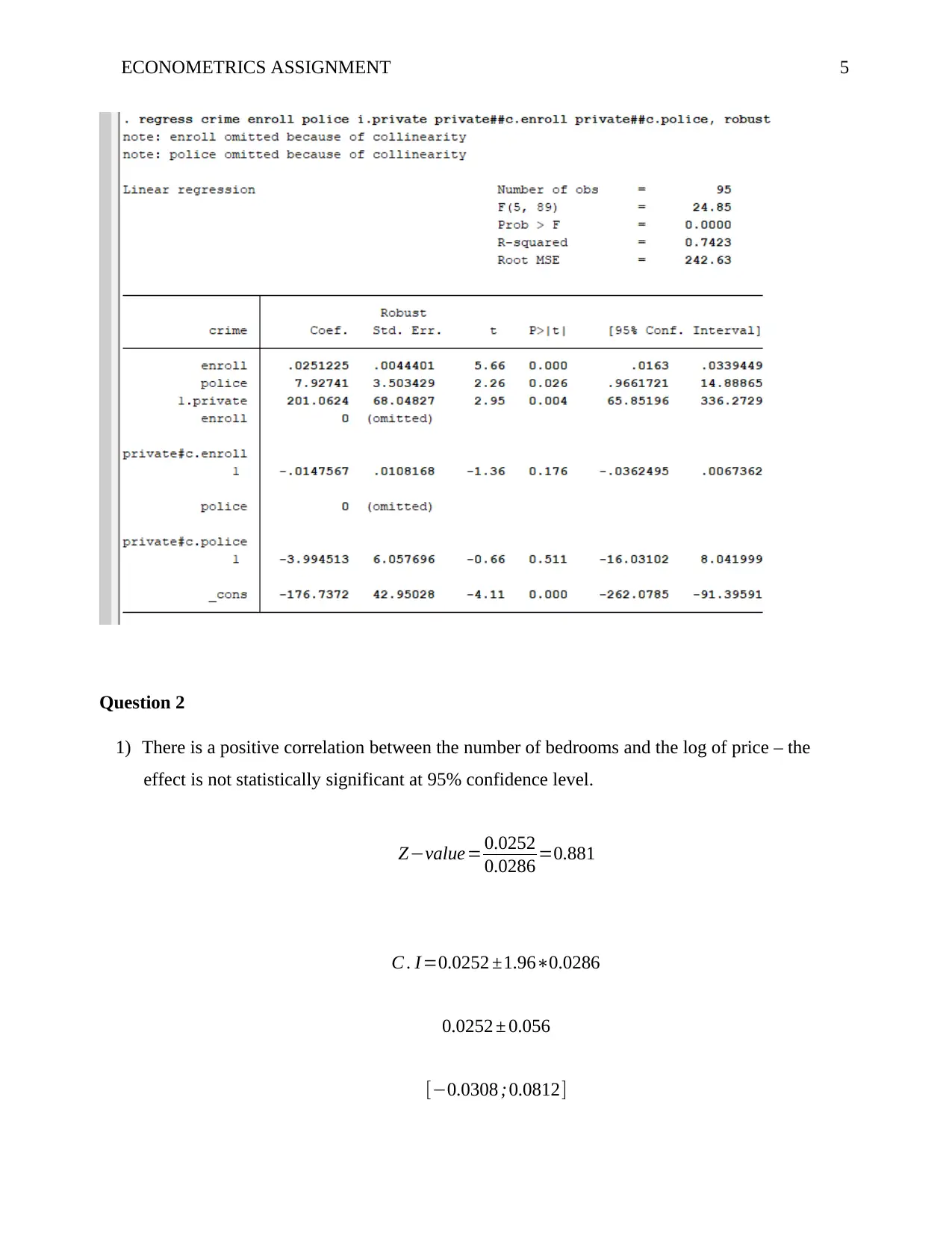
The test is significant, we conclude that there is a specification error.
9. Robust standard errors

ECONOMETRICS ASSIGNMENT 5
Question 2
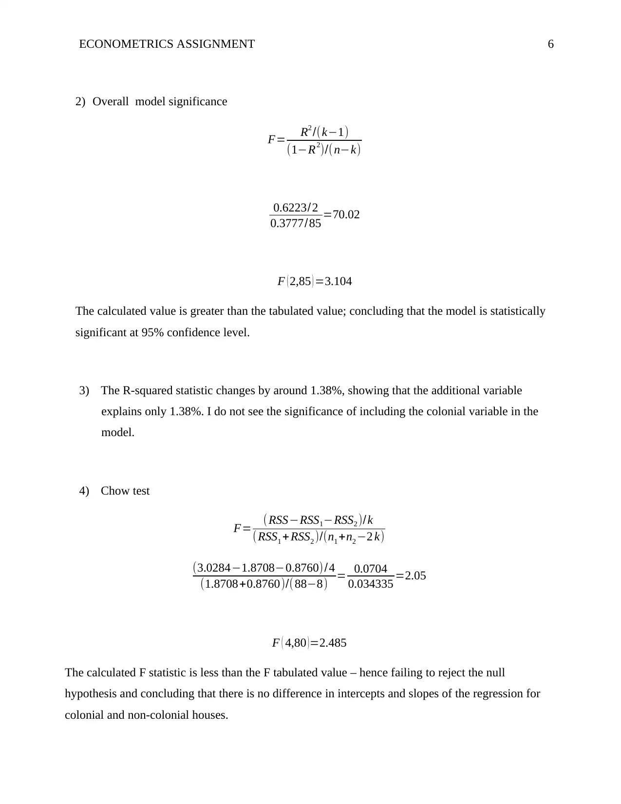
1) There is a positive correlation between the number of bedrooms and the log of price – the
effect is not statistically significant at 95% confidence level.
Z−value= 0.0252
0.0286 =0.881
C . I=0.0252 ±1.96∗0.0286
0.0252 ± 0.056
[−0.0308 ; 0.0812]

ECONOMETRICS ASSIGNMENT 6
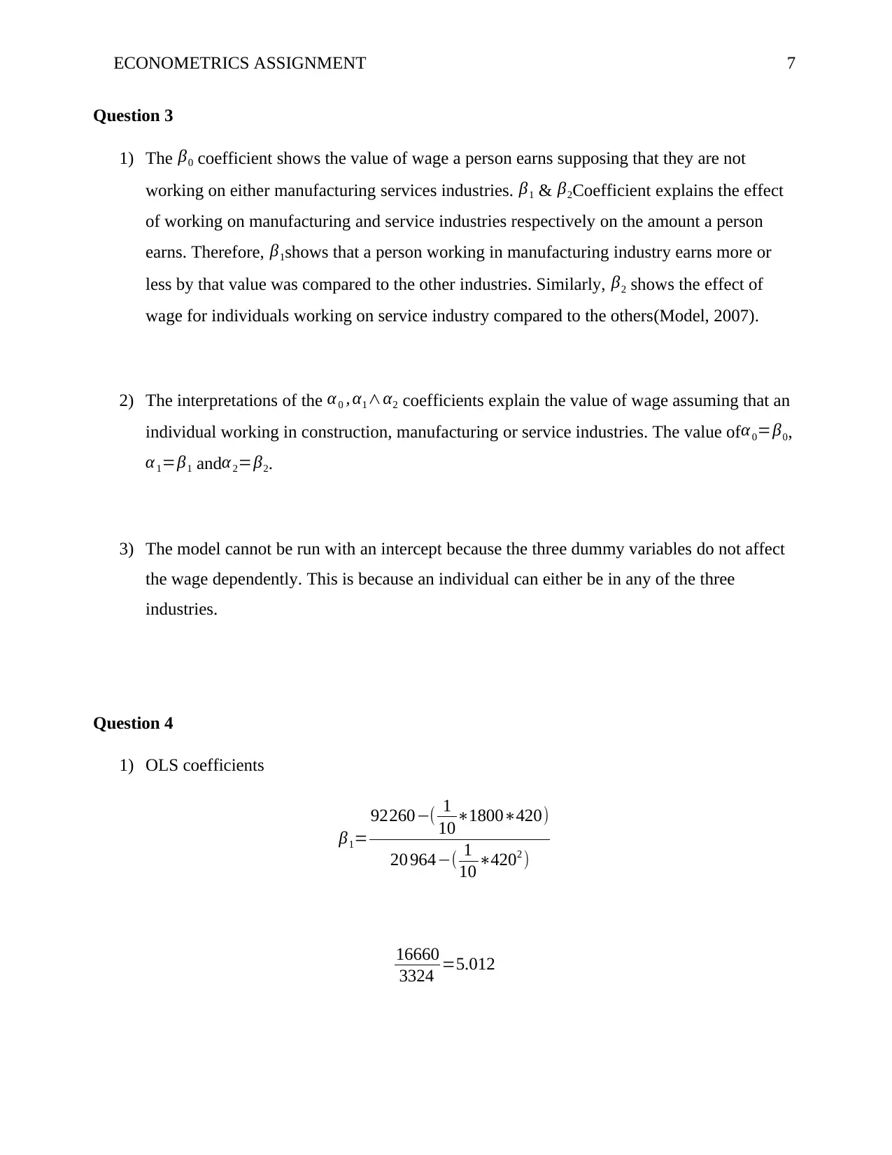
2) Overall model significance
F= R2 /(k−1)
(1−R2)/( n−k)
0.6223/2
0.3777/85 =70.02
F ( 2,85 ) =3.104
The calculated value is greater than the tabulated value; concluding that the model is statistically
significant at 95% confidence level.
3) The R-squared statistic changes by around 1.38%, showing that the additional variable
explains only 1.38%. I do not see the significance of including the colonial variable in the
model.
4) Chow test
F= ( RSS−RSS1−RSS2 )/k
(RSS1 + RSS2 )/(n1 +n2 −2 k)
(3.0284−1.8708−0.8760)/4
(1.8708+0.8760)/( 88−8) = 0.0704
0.034335 =2.05
F ( 4,80 )=2.485
The calculated F statistic is less than the F tabulated value – hence failing to reject the null
hypothesis and concluding that there is no difference in intercepts and slopes of the regression for
colonial and non-colonial houses.

ECONOMETRICS ASSIGNMENT 7
Question 3
1) The β0 coefficient shows the value of wage a person earns supposing that they are not
working on either manufacturing services industries. β1 & β2Coefficient explains the effect
of working on manufacturing and service industries respectively on the amount a person
earns. Therefore, β1shows that a person working in manufacturing industry earns more or
less by that value was compared to the other industries. Similarly, β2 shows the effect of
wage for individuals working on service industry compared to the others(Model, 2007).
2) The interpretations of the α0 , α1∧α2 coefficients explain the value of wage assuming that an
individual working in construction, manufacturing or service industries. The value of α 0=β0,
α1=β1 andα2=β2.
3) The model cannot be run with an intercept because the three dummy variables do not affect
the wage dependently. This is because an individual can either be in any of the three
industries.
Question 4
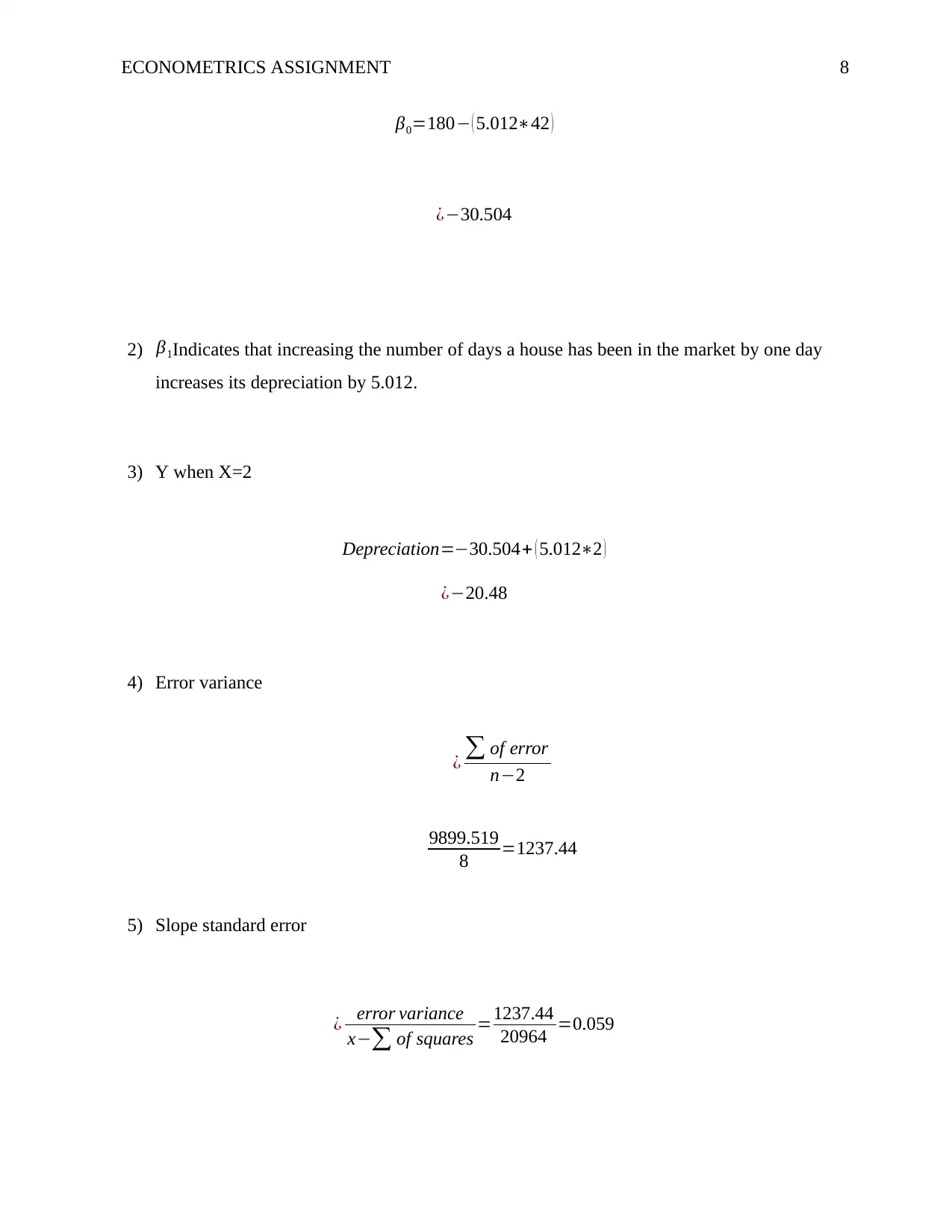
1) OLS coefficients
β1=
92260−( 1
10∗1800∗420)
20 964−( 1
10 ∗4202 )
16660
3324 =5.012

ECONOMETRICS ASSIGNMENT 8
β0=180− ( 5.012∗42 )
¿−30.504
2) β1Indicates that increasing the number of days a house has been in the market by one day
increases its depreciation by 5.012.
3) Y when X=2
Depreciation=−30.504+ ( 5.012∗2 )
¿−20.48
4) Error variance
¿ ∑ of error
n−2
9899.519
8 =1237.44
5) Slope standard error
¿ error variance
x−∑ of squares =1237.44
20964 =0.059

ECONOMETRICS ASSIGNMENT 9
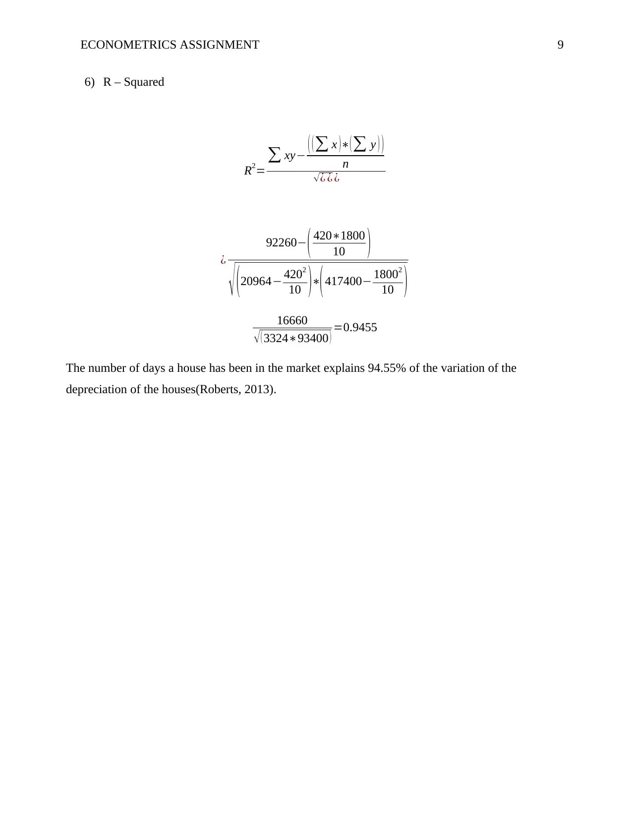
6) R – Squared
R2=
∑ xy− ( (∑ x )∗(∑ y ) )
n
√¿ ¿ ¿
¿
92260− ( 420∗1800
10 )
√ ( 20964− 4202
10 )∗( 417400− 18002
10 )
16660
√ ( 3324∗93400 ) =0.9455
The number of days a house has been in the market explains 94.55% of the variation of the
depreciation of the houses(Roberts, 2013).

ECONOMETRICS ASSIGNMENT 10
References
Fahrmeir, L., Kneib, T., Lang, S., & Marx, B. (2013). Regression : Models, Methods and
Applications. Regression.
Lynch, S. M. (2013). Introduction to multiple regression. In Using Statistics in Social Research (pp.
143–173). https://doi.org/10.1007/978-1-59745-324-0
Model, R. (2007). 7 The Linear Regression Model. Development, A167(1–2), 1–7.
https://doi.org/10.1007/0-387-22752-0_3
Roberts, D. (2013). Statistics 2 - Correlation Coefficient and Coefficient of Determination.
Retrieved from http://mathbits.com/MathBits/TISection/Statistics2/correlation.htm