Econometrics: Linear Probability Model, Logit Model, Probit Model

This document discusses the Linear Probability Model (LPM), Logit Model, and Probit Model in Econometrics. It explains the coefficients, standard errors, and how to calculate probabilities using these models. The document also includes a discussion on marginal effects in the Probit Model.

Running head: ECONOMETRICS
Econometrics
Name of the Student:
Name of the University:
Author Note:

1ECONOMETRICS
Table of Contents
Answer 1....................................................................................................................................2
Linear Probability Model (OLS)............................................................................................2
Logit Model (MLE)................................................................................................................3
Probit Model (MLE)..............................................................................................................4
Answer b....................................................................................................................................5
Marginal Effects in Probit Model..........................................................................................5
Reference:..................................................................................................................................6

2ECONOMETRICS
Answer 1
Linear Probability Model (OLS)
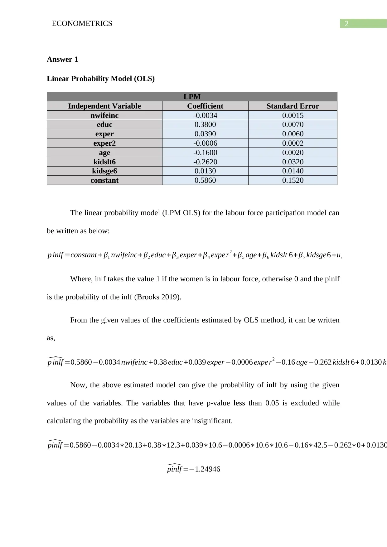
LPM
Independent Variable Coefficient Standard Error
nwifeinc -0.0034 0.0015
educ 0.3800 0.0070
exper 0.0390 0.0060
exper2 -0.0006 0.0002
age -0.1600 0.0020
kidslt6 -0.2620 0.0320
kidsge6 0.0130 0.0140
constant 0.5860 0.1520
The linear probability model (LPM OLS) for the labour force participation model can
be written as below:
p inlf =constant + β1 nwifeinc+ β2 educ + β3 exper +β4 expe r2 + β5 age+β6 kidslt 6+ β7 kidsge6 +ui
Where, inlf takes the value 1 if the women is in labour force, otherwise 0 and the pinlf
is the probability of the inlf (Brooks 2019).
From the given values of the coefficients estimated by OLS method, it can be written
as,
^p inlf =0.5860−0.0034 nwifeinc +0.38 educ +0.039 exper−0.0006 expe r2 −0.16 age−0.262 kidslt 6+ 0.0130 ki
Now, the above estimated model can give the probability of inlf by using the given
values of the variables. The variables that have p-value less than 0.05 is excluded while
calculating the probability as the variables are insignificant.
^pinlf =0.5860−0.0034∗20.13+0.38∗12.3+0.039∗10.6−0.0006∗10.6∗10.6−0.16∗42.5−0.262∗0+ 0.0130
^pinlf =−1.24946

3ECONOMETRICS
The estimated probability of being in labour force is -1.24946 which is impossible.
The result behind this weird result is the heteroscedasticity.
Logit Model (MLE)
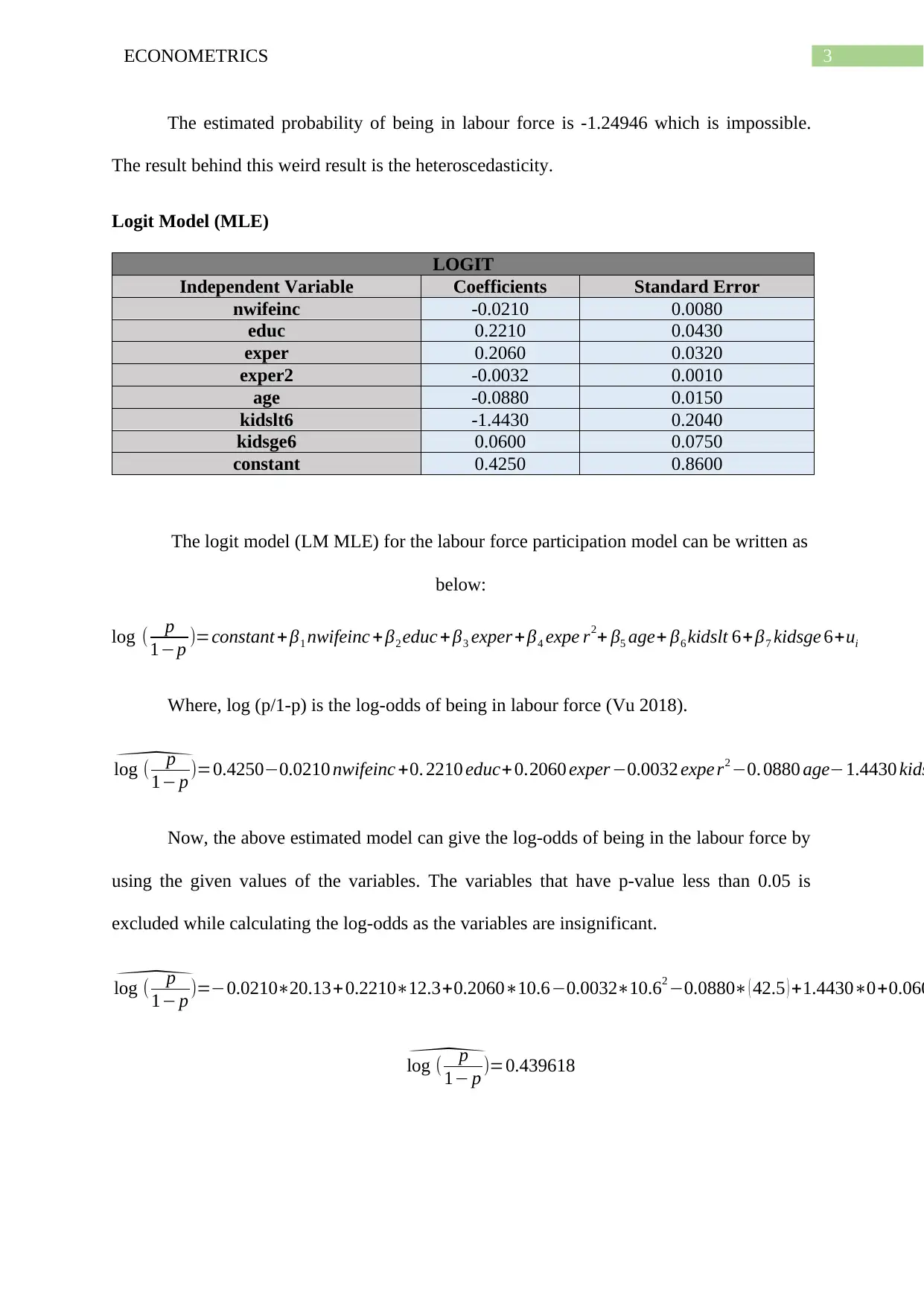
LOGIT
Independent Variable Coefficients Standard Error
nwifeinc -0.0210 0.0080
educ 0.2210 0.0430
exper 0.2060 0.0320
exper2 -0.0032 0.0010
age -0.0880 0.0150
kidslt6 -1.4430 0.2040
kidsge6 0.0600 0.0750
constant 0.4250 0.8600
The logit model (LM MLE) for the labour force participation model can be written as
below:
log ( p
1−p )=constant + β1 nwifeinc + β2 educ + β3 exper +β4 expe r2+ β5 age+ β6 kidslt 6+ β7 kidsge 6+ui
Where, log (p/1-p) is the log-odds of being in labour force (Vu 2018).
^
log ( p
1− p )=0.4250−0.0210 nwifeinc +0. 2210 educ+ 0.2060 exper−0.0032 expe r2 −0. 0880 age−1.4430 kids
Now, the above estimated model can give the log-odds of being in the labour force by
using the given values of the variables. The variables that have p-value less than 0.05 is
excluded while calculating the log-odds as the variables are insignificant.
^
log ( p
1− p )=−0.0210∗20.13+0.2210∗12.3+0.2060∗10.6−0.0032∗10.62 −0.0880∗ ( 42.5 ) +1.4430∗0+0.060
^
log ( p
1− p )=0.439618

4ECONOMETRICS
Now the probability of being in the labour force estimated by Logit model using MLE
method is equals to p= 1
1−e−0.439618 =0.608168.
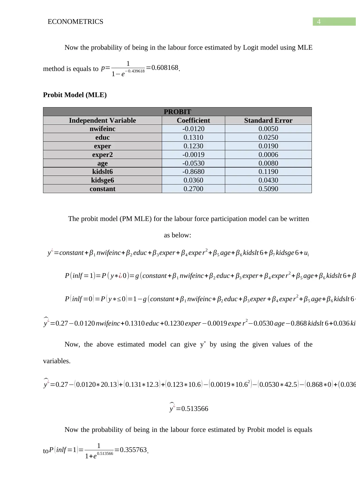
Probit Model (MLE)
PROBIT
Independent Variable Coefficient Standard Error
nwifeinc -0.0120 0.0050
educ 0.1310 0.0250
exper 0.1230 0.0190
exper2 -0.0019 0.0006
age -0.0530 0.0080
kidslt6 -0.8680 0.1190
kidsge6 0.0360 0.0430
constant 0.2700 0.5090
The probit model (PM MLE) for the labour force participation model can be written
as below:
y¿=constant + β1 nwifeinc+ β2 educ +β3 exper+ β4 expe r2 + β5 age+ β6 kidslt 6+ β7 kidsge 6+ui
P(inlf =1)=P ( y∗¿ 0)=g (constant + β1 nwifeinc+β2 educ+ β3 exper+ β4 expe r2 + β5 age+ β6 kidslt 6+ β
P ( inlf =0 ) =P ( y∗≤ 0 ) =1−g (constant +β1 nwifeinc+ β2 educ + β3 exper + β4 expe r2 + β5 age+β6 kidslt 6 +
^
y¿=0.27−0.0 120 nwifeinc+0.1310 educ +0.1230 exper−0.0019 expe r2−0.0530 age−0.868 kidslt 6+0.036 kid
Now, the above estimated model can give y* by using the given values of the
variables.
^
y¿=0.27− ( 0.0120∗20.13 )+ ( 0.131∗12.3 ) + ( 0.123∗10.6 ) − ( 0.0019∗10.62 )− ( 0.0530∗42.5 )− ( 0.868∗0 ) +(0.036
^
y¿=0.513566
Now the probability of being in the labour force estimated by Probit model is equals
toP ( inlf =1 )= 1
1+e0.513566 =0.355763.

5ECONOMETRICS
That means the data for the women indicates that the women belongs to the working
category.
Answer b
Marginal Effects in Probit Model
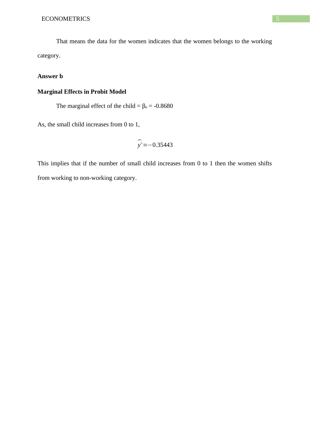
The marginal effect of the child = β6 = -0.8680
As, the small child increases from 0 to 1,
^
y¿=−0.35443
This implies that if the number of small child increases from 0 to 1 then the women shifts
from working to non-working category.

6ECONOMETRICS
Reference:
Brooks, C., 2019. Introductory econometrics for finance. Cambridge university press.
Vu, T.B., 2018. Econometrics for Daily Lives (Vol. 2). Business Expert Press.