Economic Growth and Stability: Theory and Evidence

This article discusses the theory and evidence of economic growth and stability. It covers topics such as analytical work, computational work, the golden-rule steady state, unemployment in the Solow model, and the impact of economic policies on short and long-term growth.

ECONOMIC GROWTH AND STABILITY1
Economic Growth and Stability: Theory and Evidence
Course
Instructor’s Name
Institutional Affiliation
The City and State
The Date

ECONOMIC GROWTH AND STABILITY2
Part A: Analytical Work
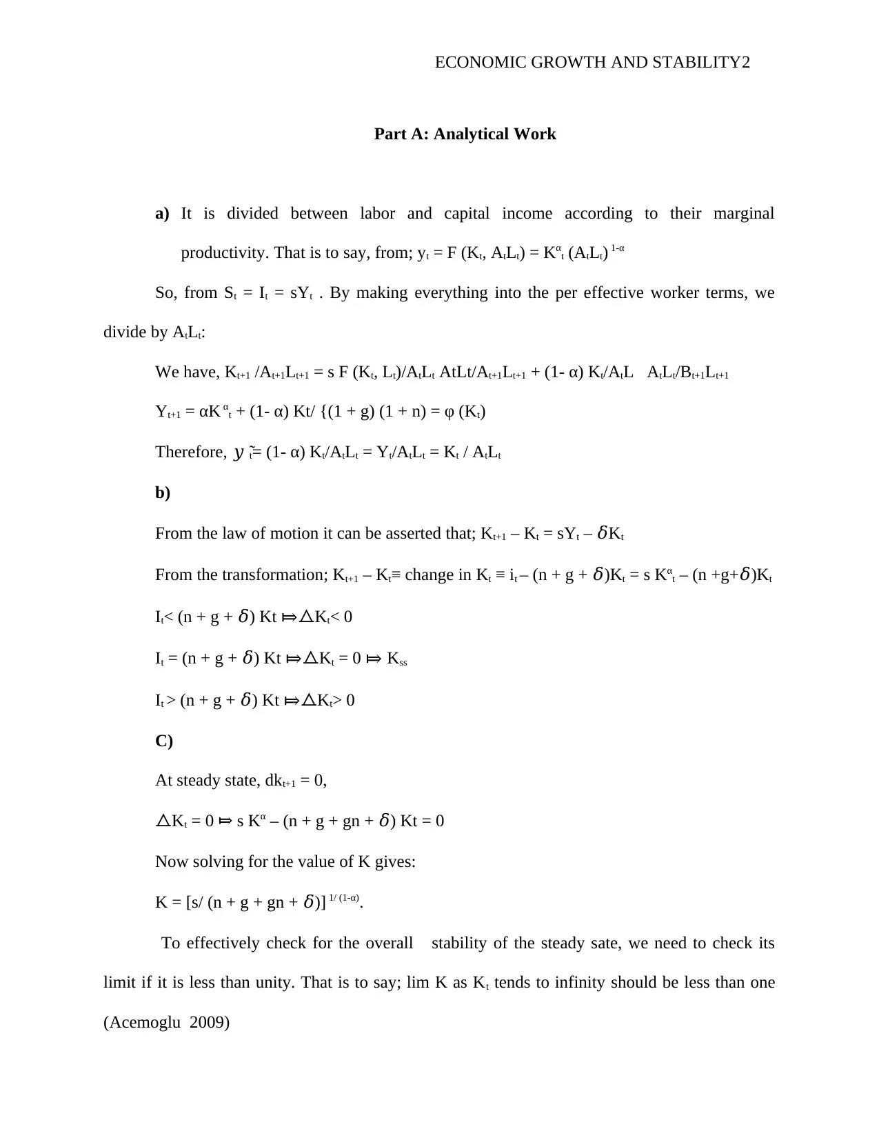
a) It is divided between labor and capital income according to their marginal
productivity. That is to say, from; yt = F (Kt, AtLt) = Kαt (AtLt) 1-α
So, from St = It = sYt . By making everything into the per effective worker terms, we
divide by AtLt:
We have, Kt+1 /At+1Lt+1 = s F (Kt, Lt)/AtLt AtLt/At+1Lt+1 + (1- α) Kt/AtL AtLt/Bt+1Lt+1
Yt+1 = αK αt + (1- α) Kt/ {(1 + g) (1 + n) = φ (Kt)
Therefore, 𝑦 ̃ t= (1- α) Kt/AtLt = Yt/AtLt = Kt / AtLt
b)
From the law of motion it can be asserted that; Kt+1 – Kt = sYt – 𝛿Kt
From the transformation; Kt+1 – Kt≡ change in Kt ≡ it – (n + g + 𝛿)Kt = s Kαt – (n +g+𝛿)Kt
It< (n + g + 𝛿) Kt ⤇⧍Kt< 0
It = (n + g + 𝛿) Kt ⤇⧍Kt = 0 ⤇ Kss
It > (n + g + 𝛿) Kt ⤇⧍Kt> 0
C)
At steady state, dkt+1 = 0,
K⧍ t = 0 s K⤇ α – (n + g + gn + 𝛿) Kt = 0
Now solving for the value of K gives:
K = [s/ (n + g + gn + 𝛿)] 1/ (1-α).
To effectively check for the overall stability of the steady sate, we need to check its
limit if it is less than unity. That is to say; lim K as Kt tends to infinity should be less than one
(Acemoglu 2009)

ECONOMIC GROWTH AND STABILITY3
For output per worker
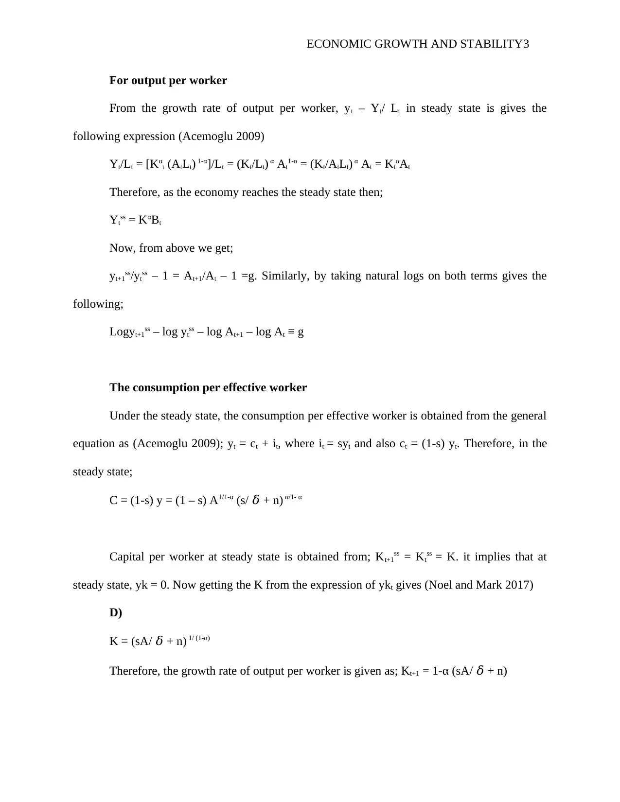
From the growth rate of output per worker, yt – Yt/ Lt in steady state is gives the
following expression (Acemoglu 2009)
Yt/Lt = [Kαt (AtLt) 1-α]/Lt = (Kt/Lt) α At1-α = (Kt/AtLt) α At = KtαAt
Therefore, as the economy reaches the steady state then;
Ytss = KαBt
Now, from above we get;
yt+1ss/ytss – 1 = At+1/At – 1 =g. Similarly, by taking natural logs on both terms gives the
following;
Logyt+1ss – log ytss – log At+1 – log At ≡ g
The consumption per effective worker
Under the steady state, the consumption per effective worker is obtained from the general
equation as (Acemoglu 2009); yt = ct + it, where it = syt and also ct = (1-s) yt. Therefore, in the
steady state;
C = (1-s) y = (1 – s) A1/1-α (s/ 𝛿 + n) α/1- α
Capital per worker at steady state is obtained from; Kt+1ss = Ktss = K. it implies that at
steady state, yk = 0. Now getting the K from the expression of ykt gives (Noel and Mark 2017)
D)
K = (sA/ 𝛿 + n) 1/ (1-α)
Therefore, the growth rate of output per worker is given as; Kt+1 = 1-α (sA/ 𝛿 + n)

ECONOMIC GROWTH AND STABILITY4
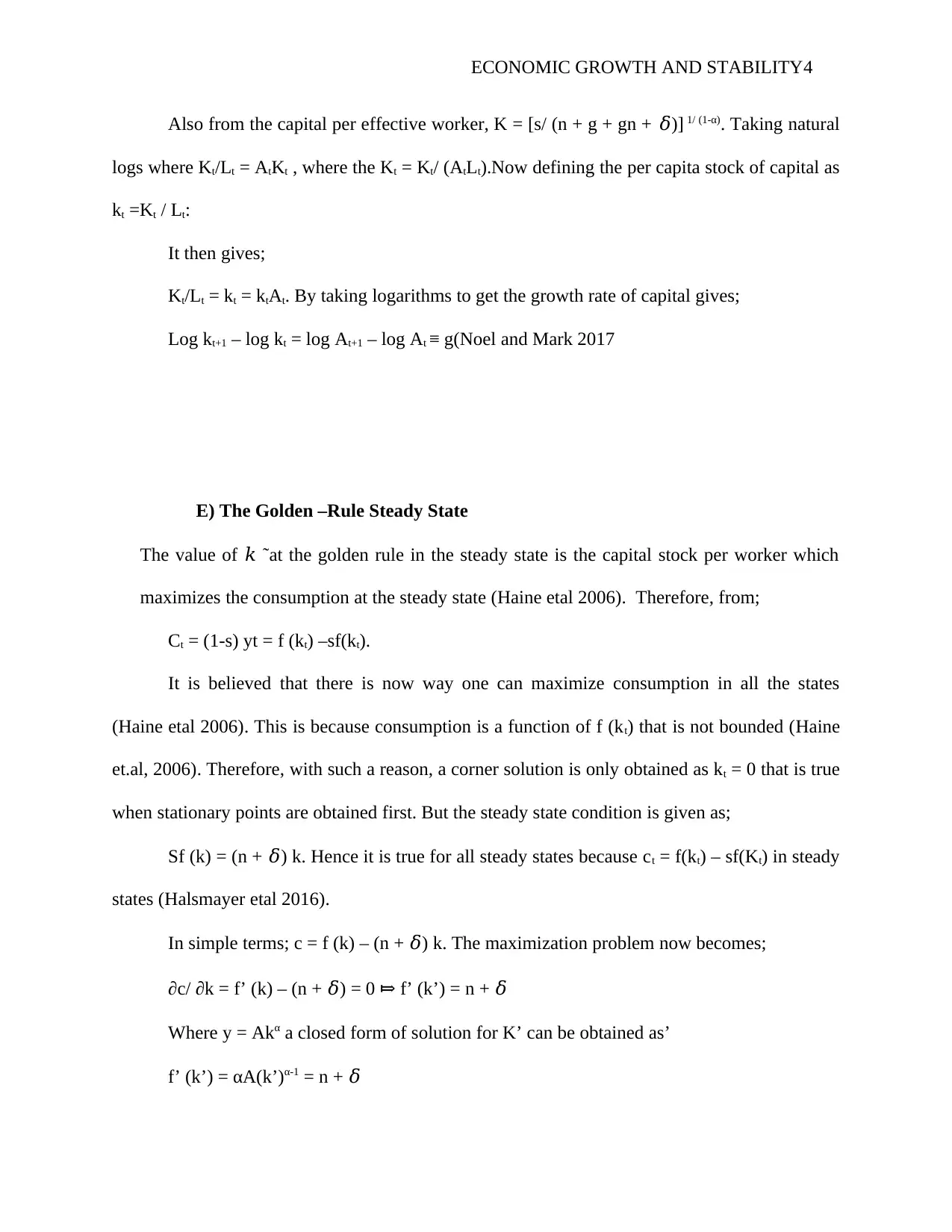
Also from the capital per effective worker, K = [s/ (n + g + gn + 𝛿)] 1/ (1-α). Taking natural
logs where Kt/Lt = AtKt , where the Kt = Kt/ (AtLt).Now defining the per capita stock of capital as
kt =Kt / Lt:
It then gives;
Kt/Lt = kt = ktAt. By taking logarithms to get the growth rate of capital gives;
Log kt+1 – log kt = log At+1 – log At ≡ g(Noel and Mark 2017
E) The Golden –Rule Steady State
The value of 𝑘 ̃ at the golden rule in the steady state is the capital stock per worker which
maximizes the consumption at the steady state (Haine etal 2006). Therefore, from;
Ct = (1-s) yt = f (kt) –sf(kt).
It is believed that there is now way one can maximize consumption in all the states
(Haine etal 2006). This is because consumption is a function of f (kt) that is not bounded (Haine
et.al, 2006). Therefore, with such a reason, a corner solution is only obtained as kt = 0 that is true
when stationary points are obtained first. But the steady state condition is given as;
Sf (k) = (n + 𝛿) k. Hence it is true for all steady states because ct = f(kt) – sf(Kt) in steady
states (Halsmayer etal 2016).
In simple terms; c = f (k) – (n + 𝛿) k. The maximization problem now becomes;
∂c/ ∂k = f’ (k) – (n + 𝛿) = 0 f’ (k’) = n +⤇ 𝛿
Where y = Akα a closed form of solution for K’ can be obtained as’
f’ (k’) = αA(k’)α-1 = n + 𝛿

ECONOMIC GROWTH AND STABILITY5
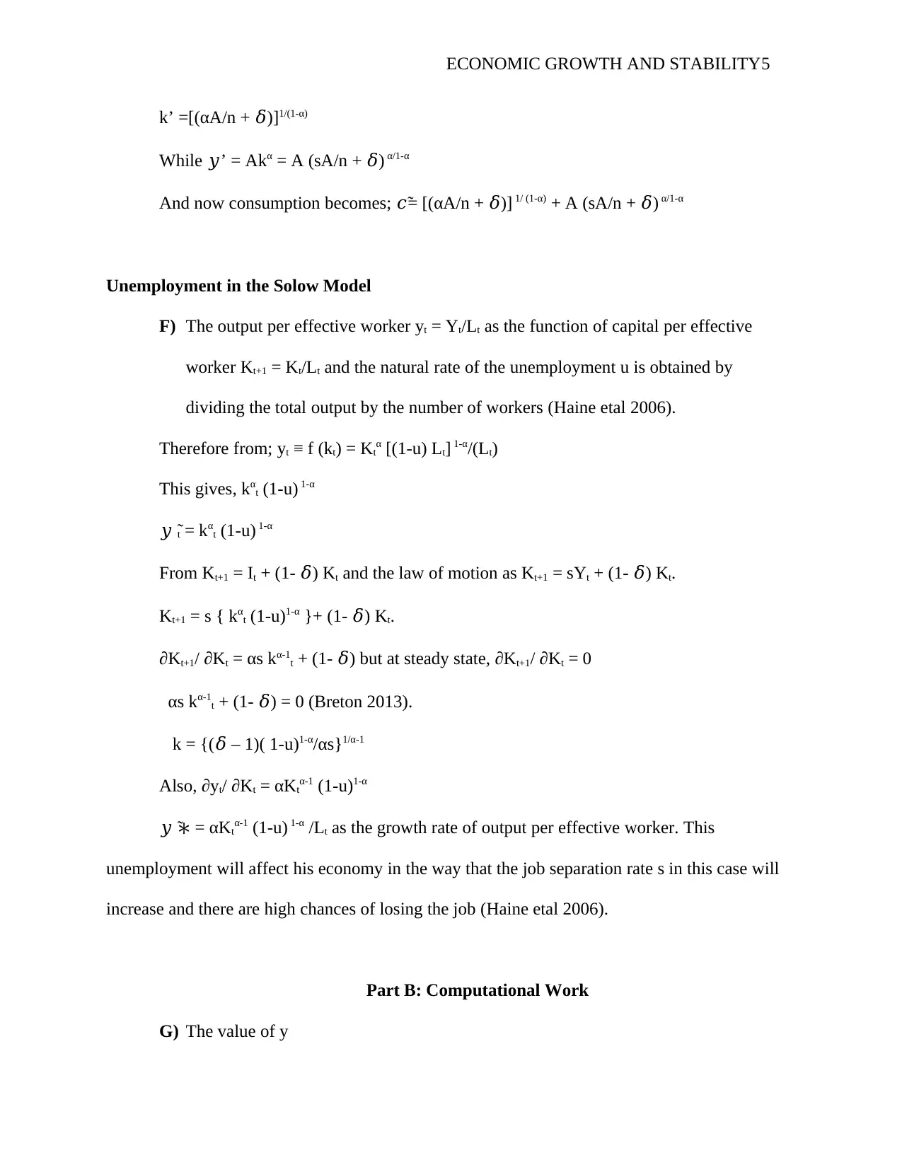
k’ =[(αA/n + 𝛿)]1/(1-α)
While 𝑦’ = Akα = A (sA/n + 𝛿) α/1-α
And now consumption becomes; 𝑐̃= [(αA/n + 𝛿)] 1/ (1-α) + A (sA/n + 𝛿) α/1-α
Unemployment in the Solow Model
F) The output per effective worker yt = Yt/Lt as the function of capital per effective
worker Kt+1 = Kt/Lt and the natural rate of the unemployment u is obtained by
dividing the total output by the number of workers (Haine etal 2006).
Therefore from; yt ≡ f (kt) = Ktα [(1-u) Lt] 1-α/(Lt)
This gives, kαt (1-u) 1-α
𝑦 ̃ t = kαt (1-u) 1-α
From Kt+1 = It + (1- 𝛿) Kt and the law of motion as Kt+1 = sYt + (1- 𝛿) Kt.
Kt+1 = s { kαt (1-u)1-α }+ (1- 𝛿) Kt.
∂Kt+1/ ∂Kt = αs kα-1t + (1- 𝛿) but at steady state, ∂Kt+1/ ∂Kt = 0
αs kα-1t + (1- 𝛿) = 0 (Breton 2013).
k = {(𝛿 – 1)( 1-u)1-α/αs}1/α-1
Also, ∂yt/ ∂Kt = αKtα-1 (1-u)1-α
𝑦 ̃ ∗ = αKtα-1 (1-u) 1-α /Lt as the growth rate of output per effective worker. This
unemployment will affect his economy in the way that the job separation rate s in this case will
increase and there are high chances of losing the job (Haine etal 2006).
Part B: Computational Work
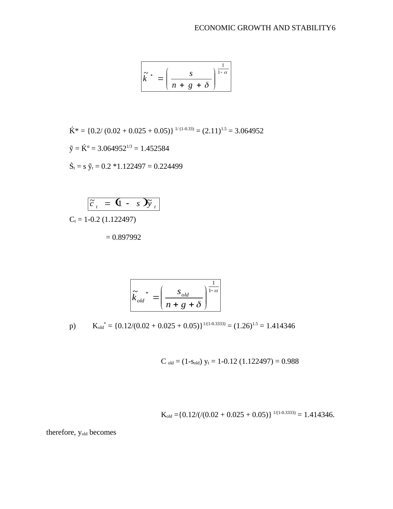
G) The value of y

ECONOMIC GROWTH AND STABILITY6
Ḱ* = {0.2/ (0.02 + 0.025 + 0.05)} 1/ (1-0.33) = (2.11)1.5 = 3.064952
ỹ = Ḱα = 3.0649521/3 = 1.452584
Ṡt = s ỹt = 0.2 *1.122497 = 0.224499
Ct = 1-0.2 (1.122497)
= 0.897992
p) Kold* = {0.12/(0.02 + 0.025 + 0.05)}1/(1-0.3333) = (1.26)1.5 = 1.414346
C old = (1-sold) yt = 1-0.12 (1.122497) = 0.988
Kold ={0.12/(/(0.02 + 0.025 + 0.05)} 1/(1-0.3333) = 1.414346.
therefore, yold becomes










 1
1
*~
gn
s
k
  tt ysc ~1~ 










 1
1
*~
gn
s
k old
old

ECONOMIC GROWTH AND STABILITY7
Yold= Ḱα = 1.4143461/3 = 1.122497
-4.00000000000
-2.00000000000
0.00000000000
2.00000000000
4.00000000000
6.00000000000
8.00000000000
10.00000000000
12.00000000000
14.00000000000
1
19
37
55
73
91
109
127
145
163
181
199
217
235
253
271
289
k~_t
y~_t
s~_t
c~_t
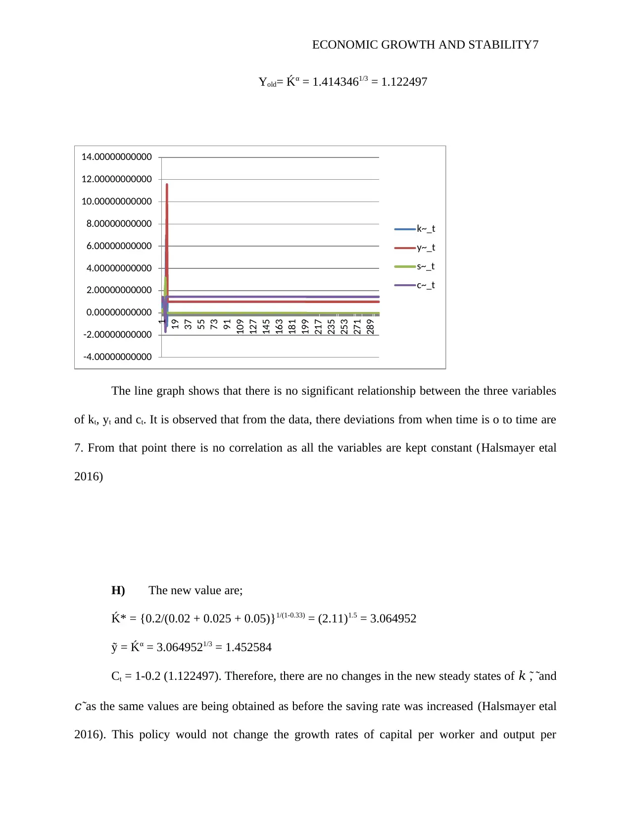
The line graph shows that there is no significant relationship between the three variables
of kt, yt and ct. It is observed that from the data, there deviations from when time is o to time are
7. From that point there is no correlation as all the variables are kept constant (Halsmayer etal
2016)
H) The new value are;
Ḱ* = {0.2/(0.02 + 0.025 + 0.05)}1/(1-0.33) = (2.11)1.5 = 3.064952
ỹ = Ḱα = 3.0649521/3 = 1.452584
Ct = 1-0.2 (1.122497). Therefore, there are no changes in the new steady states of 𝑘 ̃ , ̃ and
𝑐̃ as the same values are being obtained as before the saving rate was increased (Halsmayer etal
2016). This policy would not change the growth rates of capital per worker and output per

ECONOMIC GROWTH AND STABILITY8
worker. This is because there the policy has no effect on the steady states of 𝑘 ̃ , ̃ and 𝑐̃.
However, in the short run, consumption reduces with time as saving increases. This is explained
since saving increases, this would imply that, consumption in the short run will also reduce and
finally no consumption at all in the long run (Halsmayer etal 2016).
I) The impact of this policy in the short run is that, consumption is not affected but
saving increases and capital ratio slightly falls. While in the long run, most of the
variables are seen to change like the consumption which declines heavily and also
capital ratio reduces as investment increases as a result of saving (Halsmayer et al
2016).
-5.000000000
0.000000000
5.000000000
10.000000000
15.000000000
20.000000000
25.000000000
30.000000000
35.000000000
1.452578475
0.000000000
1.000000000
1.000000000
1.000000000
1.000000000
1.000000000
1.000000000
1.000000000
1.000000000
1.000000000
1.000000000
1.000000000
1.000000000
1.228079475
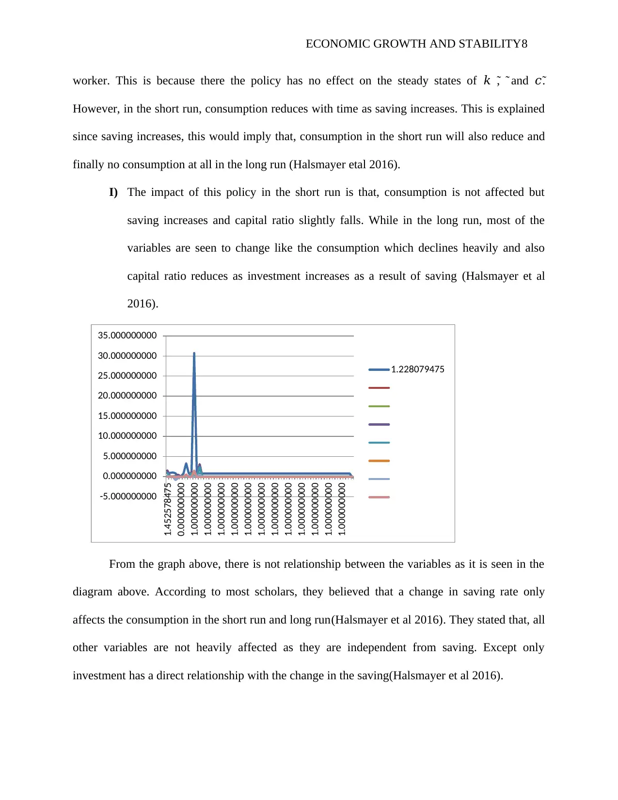
From the graph above, there is not relationship between the variables as it is seen in the
diagram above. According to most scholars, they believed that a change in saving rate only
affects the consumption in the short run and long run(Halsmayer et al 2016). They stated that, all
other variables are not heavily affected as they are independent from saving. Except only
investment has a direct relationship with the change in the saving(Halsmayer et al 2016).

ECONOMIC GROWTH AND STABILITY9
Part C: A Contribution to the Empirics of Economic Growth. Solow Model with Human
Capital
J) It is believed that the Solow Model is built upon the neoclassical dynamic model with the
aggregate production function (Halsmayer et al 2016).
From the general equation as, Y (t) = [A (t), K (t), L (t)]………………………….1
Where the Y (t) is the aggregate output at time t, output is then presented as the function
of the capital inputs (Halsmayer etal2016). From the same equation, the households have got
capital that is available for renting to other individuals and firms which depreciates at (𝛿).
Therefore, the net change of capital is obtained from the following equation;
Ḱ = sY – 𝛿K…………………………………………………..2
Where Ḱ presents the time derivatives. Firms under Solow aim at profit maximization.
Also from the Solow model, the neoclassical production is obtained from the Cobb Douglas
functions as (Halsmayer et al 2016);
Y(t) = A(t)K(t)αL(t)1-α, that is to say; 0<α<1 where α is the output share paid to the capital
while 1- α is the output share that is paid to the labor. When labor productivity is increased by
the presence of technology, the function becomes;
q) Y(t) = K(t)α(A(t)L(t))1-α …………………………………..3. Where A (t) L (t) is
the labor effective. Then when A is expressed as the factor which increases labor productivity,
we obtain income per unit of effective labor as a function of the capital per unit of effective labor
as given by; (Noel and Mark 2017)
r) (Y(t)/A(t)L(t)={k/(A(t)L(t))}α*{A(t)L(t)/(A(t)L(t)}1α⤇y=Kα…4. where y is the
output per unit of the effective labor while k is the capital per unit of effective labor. However,
any changes in capital will lead to changes in the level of total income as determined by;

ECONOMIC GROWTH AND STABILITY10
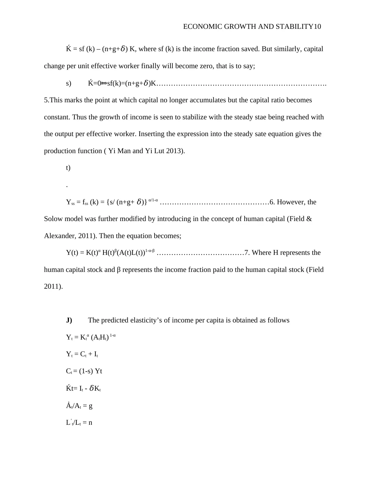
Ḱ = sf (k) – (n+g+𝛿) K, where sf (k) is the income fraction saved. But similarly, capital
change per unit effective worker finally will become zero, that is to say;
s) Ḱ=0 sf(k)=(n+g+⤇ 𝛿)K…………………………………………………………….
5.This marks the point at which capital no longer accumulates but the capital ratio becomes
constant. Thus the growth of income is seen to stabilize with the steady stae being reached with
the output per effective worker. Inserting the expression into the steady sate equation gives the
production function ( Yi Man and Yi Lut 2013).
t)
.
Yss = fss (k) = {s/ (n+g+ 𝛿)} α/1-α ………………………………………6. However, the
Solow model was further modified by introducing in the concept of human capital (Field &
Alexander, 2011). Then the equation becomes;
Y(t) = K(t)α H(t)β(A(t)L(t))1-α-β ………………………………7. Where H represents the
human capital stock and β represents the income fraction paid to the human capital stock (Field
2011).
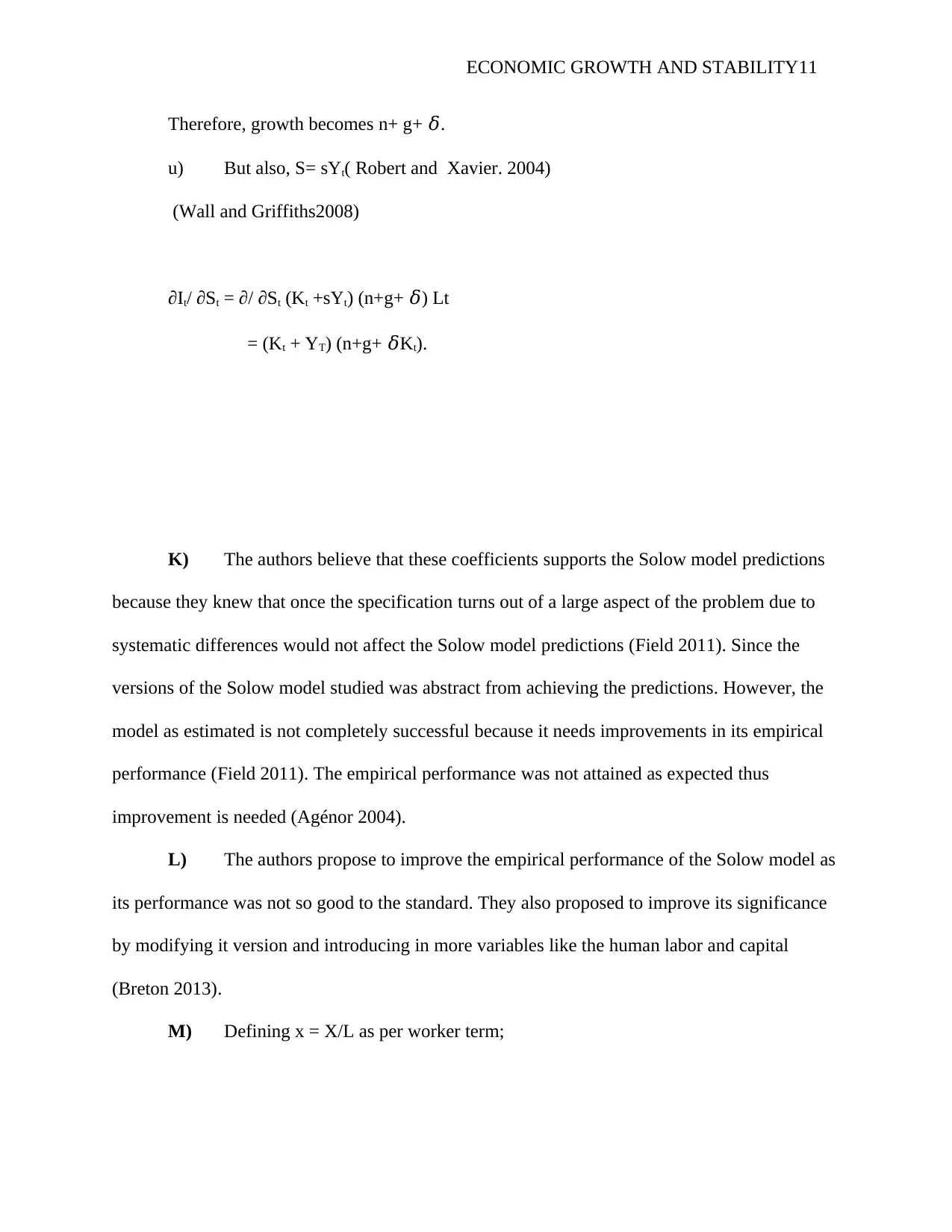
J) The predicted elasticity’s of income per capita is obtained as follows
Yt = Ktα (AtHt) 1-α
Yt = Ct + It
Ct = (1-s) Yt
Ḱt= It - 𝛿Kt
Ảt/At = g
L’t/Lt = n

ECONOMIC GROWTH AND STABILITY11
Therefore, growth becomes n+ g+ 𝛿.
u) But also, S= sYt( Robert and Xavier. 2004)
(Wall and Griffiths2008)
∂It/ ∂St = ∂/ ∂St (Kt +sYt) (n+g+ 𝛿) Lt
= (Kt + YT) (n+g+ 𝛿Kt).
K) The authors believe that these coefficients supports the Solow model predictions
because they knew that once the specification turns out of a large aspect of the problem due to
systematic differences would not affect the Solow model predictions (Field 2011). Since the
versions of the Solow model studied was abstract from achieving the predictions. However, the
model as estimated is not completely successful because it needs improvements in its empirical
performance (Field 2011). The empirical performance was not attained as expected thus
improvement is needed (Agénor 2004).
L) The authors propose to improve the empirical performance of the Solow model as
its performance was not so good to the standard. They also proposed to improve its significance
by modifying it version and introducing in more variables like the human labor and capital
(Breton 2013).
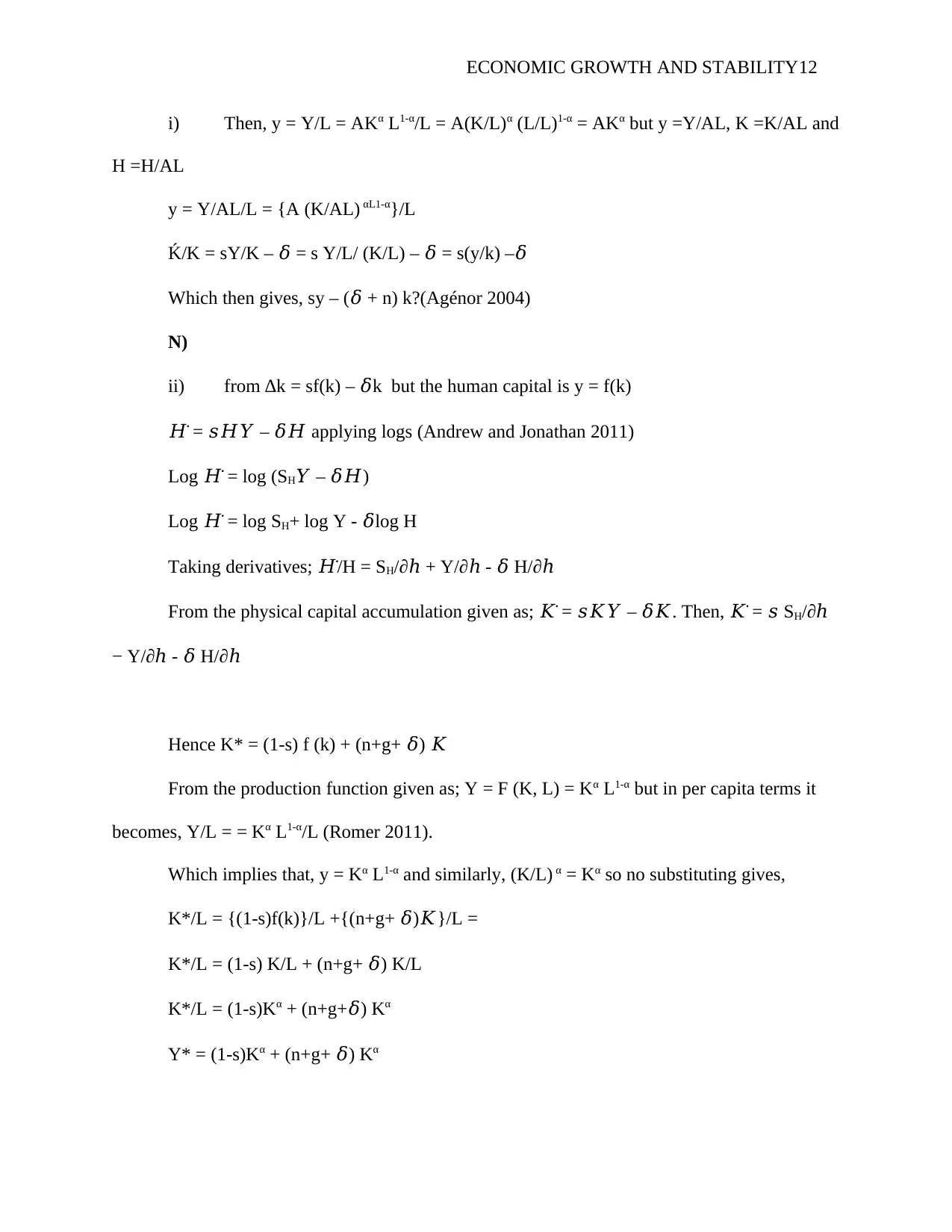
M) Defining x = X/L as per worker term;

ECONOMIC GROWTH AND STABILITY12
i) Then, y = Y/L = AKα L1-α/L = A(K/L)α (L/L)1-α = AKα but y =Y/AL, K =K/AL and
H =H/AL
y = Y/AL/L = {A (K/AL) αL1-α}/L
Ḱ/K = sY/K – 𝛿 = s Y/L/ (K/L) – 𝛿 = s(y/k) –𝛿
Which then gives, sy – (𝛿 + n) k?(Agénor 2004)
N)
ii) from ∆k = sf(k) – 𝛿k but the human capital is y = f(k)
𝐻̇ = 𝑠𝐻𝑌 – 𝛿𝐻 applying logs (Andrew and Jonathan 2011)
Log 𝐻̇ = log (SH𝑌 – 𝛿𝐻)
Log 𝐻̇ = log SH+ log Y - 𝛿log H
Taking derivatives; 𝐻̇/H = SH/∂ℎ + Y/∂ℎ - 𝛿 H/∂ℎ
From the physical capital accumulation given as; 𝐾̇ = 𝑠𝐾𝑌 – 𝛿𝐾. Then, 𝐾̇ = 𝑠 SH/∂ℎ
− Y/∂ -ℎ 𝛿 H/∂ℎ
Hence K* = (1-s) f (k) + (n+g+ 𝛿) 𝐾
From the production function given as; Y = F (K, L) = Kα L1-α but in per capita terms it
becomes, Y/L = = Kα L1-α/L (Romer 2011).
Which implies that, y = Kα L1-α and similarly, (K/L) α = Kα so no substituting gives,
K*/L = {(1-s)f(k)}/L +{(n+g+ 𝛿)𝐾}/L =
K*/L = (1-s) K/L + (n+g+ 𝛿) K/L
K*/L = (1-s)Kα + (n+g+𝛿) Kα
Y* = (1-s)Kα + (n+g+ 𝛿) Kα

ECONOMIC GROWTH AND STABILITY13
O) The author used 𝑠𝐻 in his equation simply because he wanted to account for the changes in
share of capital. The authors realized that there are variations in the share of capital and so to
account for them the 𝑠𝐻 was introduced (Romer 2011)
p). The results of estimating eq. (11) show that there is an increase in the share of capital as
𝑠𝐻 was introduced which caused a fall in the human capital. The Authors are sure that this
equation is best to fit for the data because the biasness was removed by introducing the 𝑠𝐻
into the equation. Therefore, the equation would produce more realistic results once it is
fitted for the data (Breton 2013).

ECONOMIC GROWTH AND STABILITY14
References
Acemoglu, Daron. 2009. "The Solow Growth Model". Introduction to Modern Economic
Growth. Princeton: Princeton University Press. pp. 26–76. Accessed 12 Oct.2018.
Haines, Joel D.; Sharif, Nawaz M. 2006. "A framework for managing the sophistication of the
components of technology for global competition". Competitiveness Review: An
International Business Journal. Emerald. Vol 16 (2). Pp 106–121.
doi:10.1108/cr.2006.16.2.106.
Halsmayer, Verena; Hoover, Kevin D. 2016. "Solow's Harrod: Transforming macroeconomic
dynamics into a model of long-run growth". The European Journal of the History of
Economic Thought. 23 (4): 561–596. doi:10.1080/09672567.2014.1001763. Accessed on
12 October 2018
Romer, D. 2011. "The Solow Growth Model". Advanced Macroeconomics (Fourth ed.). New
York: McGraw-Hill. pp. 6–48. Accessed on 12 October 2018.
Agénor, Pierre-Richard. 2004. "Growth and Technological Progress: The Solow–Swan Model".
The Economics of Adjustment and Growth (Second ed.). Cambridge: Harvard University
Press. pp. 439–462. Accessed on 12 October 2018
Barro, Robert J.; Sala-i-Martin, Xavier. 2004. "Growth Models with Exogenous Saving Rates".
Economic Growth (Second ed.). New York: McGraw-Hill. pp. 23–84. Accessed on 12
October 2018

ECONOMIC GROWTH AND STABILITY15
Field, A. J. 2011. A Great Leap Forward: 1930s Depression and U.S. Economic Growth. New
Haven, London: Yale University Press. Accessed on 12 October 2018
Li, Rita Yi Man; Li, Yi Lut. 2013. "Is There a Positive Relationship between Law and Economic
Growth? A Paradox in China". Asian Social Science. 9 (9): 19–30. Accessed on 12
October 2018
Johnson, Noel D.; Koyama, Mark (2017). "States and Economic Growth: Capacity and
Constraints". Explorations in Economic History. Vol 64. Pp 1–20.
doi:10.1016/j.eeh.2016.11.002.
Berg, Andrew G.; Ostry, Jonathan D. 2011. "Equality and Efficiency". Finance and
Development. International Monetary Fund. Vol 48 (3). Retrieved on 12 October 2018.
Field, A. J. 2011. A Great Leap Forward: 1930s Depression and U.S. Economic Growth. New
Haven, London: Yale University Press. Accessed on 12 October 2018.
Johnson, Noel D.; Koyama, Mark. 2017. "States and Economic Growth: Capacity and
Constraints". Explorations in Economic History. 64: 1–20. doi:10.1016/j.eeh.2016.11.002
Breton, T. R. 2013. "The role of education in economic growth: Theory, history and current
returns". Educational Research. 55 (2): 121. doi:10.1080/00131881.2013.801241.
Wall, S.; Griffiths, A. 2008. Economics for Business and Management. Financial Times Prentice
Hall. ISBN 978-0-273-71367-8. Retrieved 6 March
2010.https://books.google.com/books? Id=TrRtUr_Wn2IC