Economics Report: Comparative Analysis of Financial Markets

This economics report presents a detailed analysis of the AUD/USD currency pair, Bitcoin, and coal prices over a two-year period. It begins by visualizing the continuously compounded returns of AUD/USD and examining its distributional features, including skewness and kurtosis, in relation to a normal distribution. The report then assesses the volatility of the currency pair and projects its directional movement using statistical methods. A comparative analysis of volatility and return distribution is conducted between AUD/USD and Bitcoin, evaluating Bitcoin's characteristics as a legitimate currency. Finally, the report measures the correlation between AUD and coal prices, discussing the concept of commodity currencies and their economic implications, supported by relevant third-party research and data.

Running head: ECONOMICS
Economics
Name of the Student:
Name of the University:
Author’s Note:

1ECONOMICS
Table of Contents
Question 1........................................................................................................................................2
Question 2........................................................................................................................................3
Question 3........................................................................................................................................5
Question 4........................................................................................................................................6
Question 5........................................................................................................................................7
Question 6........................................................................................................................................7
References......................................................................................................................................11

2ECONOMICS
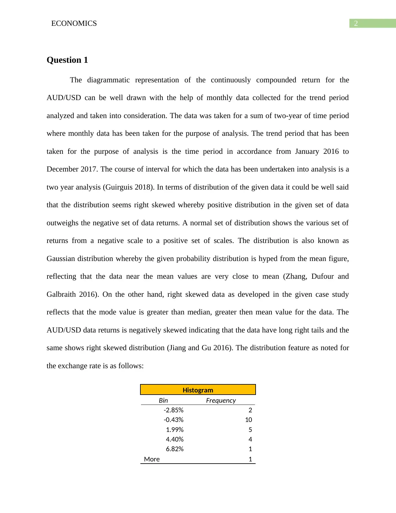
Question 1
The diagrammatic representation of the continuously compounded return for the
AUD/USD can be well drawn with the help of monthly data collected for the trend period
analyzed and taken into consideration. The data was taken for a sum of two-year of time period
where monthly data has been taken for the purpose of analysis. The trend period that has been
taken for the purpose of analysis is the time period in accordance from January 2016 to
December 2017. The course of interval for which the data has been undertaken into analysis is a
two year analysis (Guirguis 2018). In terms of distribution of the given data it could be well said
that the distribution seems right skewed whereby positive distribution in the given set of data
outweighs the negative set of data returns. A normal set of distribution shows the various set of
returns from a negative scale to a positive set of scales. The distribution is also known as
Gaussian distribution whereby the given probability distribution is hyped from the mean figure,
reflecting that the data near the mean values are very close to mean (Zhang, Dufour and
Galbraith 2016). On the other hand, right skewed data as developed in the given case study
reflects that the mode value is greater than median, greater then mean value for the data. The
AUD/USD data returns is negatively skewed indicating that the data have long right tails and the
same shows right skewed distribution (Jiang and Gu 2016). The distribution feature as noted for
the exchange rate is as follows:
Histogram
Bin Frequency
-2.85% 2
-0.43% 10
1.99% 5
4.40% 4
6.82% 1
More 1

3ECONOMICS
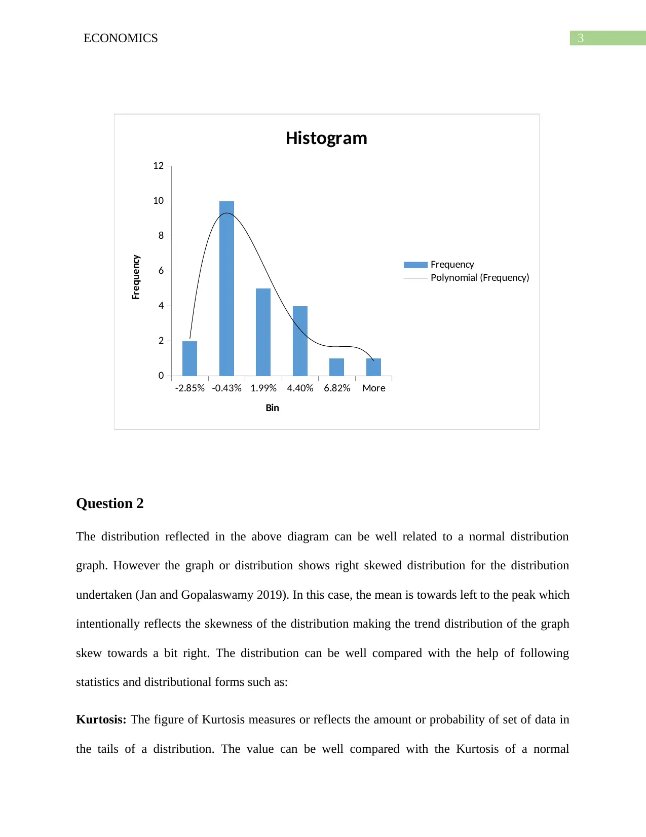
-2.85% -0.43% 1.99% 4.40% 6.82% More
0
2
4
6
8
10
12
Histogram
Frequency
Polynomial (Frequency)
Bin
Frequency
Question 2
The distribution reflected in the above diagram can be well related to a normal distribution
graph. However the graph or distribution shows right skewed distribution for the distribution
undertaken (Jan and Gopalaswamy 2019). In this case, the mean is towards left to the peak which
intentionally reflects the skewness of the distribution making the trend distribution of the graph
skew towards a bit right. The distribution can be well compared with the help of following
statistics and distributional forms such as:
Kurtosis: The figure of Kurtosis measures or reflects the amount or probability of set of data in
the tails of a distribution. The value can be well compared with the Kurtosis of a normal

4ECONOMICS
distribution which has been equal to 3 (Jammazi Lahiani and Nguyen 2015). If the figure
determined for Kurtosis is greater than 3, then the data set can be said to have a heavier tails
other than a normal distributions. In the case of data evaluated here the value of Kurtosis
determined was around 0.21 and the same says that the value is comparatively less in the tails of
the distributions drawn. The Kurtosis figure here is very low which shows that the tail risk is
comparatively lower for the data set of distributions analyzed. The median and mode figures are
comparatively higher in this set of data.
Skewness: In the theory of probability it can be well said that the skewness is a measure of
asymmetry of probability distribution of a real valued random variable in accordance with the
mean value. The value of skewness can be positive, negative and the same even can be
undefined. If the level of skewness in the set of data undertaken is less than -1 or greater than 1,
the distribution analyzed can be said to be highly skewed. If the level of skewness is between -1
and -0.5 or between 0.5 and 1, the distribution can be well described as moderately skewed. The
data analyzed shows a moderate skewed distribution for the data as the skewness was around
0.54.
The results of descriptive set of data analyzed for the exchange rate is as follows:
Column1
Mean 0.004592858
Standard Error 0.006015026
Median -0.006997376
Mode #N/A
Standard Deviation 0.028847049
Sample Variance 0.000832152
Kurtosis 0.021888734
Skewness 0.543716568
Range 0.12091367
Minimum -0.048665001

5ECONOMICS
Maximum 0.07224867
Sum 0.105635731
Count 23
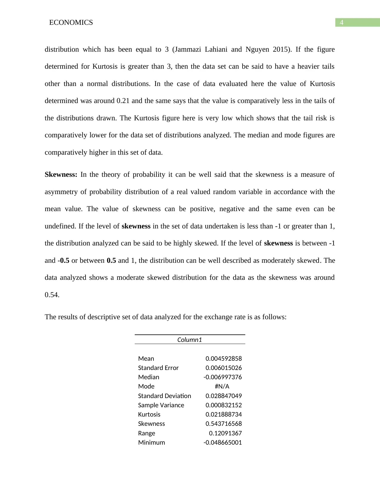
Question 3
Volatility in the set of given data can be well explained with the help of movement of
various factors that can explain the movement in the trend period analyzed for the exchange rate
between 2016-2017. The volatility or the standard deviation could be calculated with the help of
the movement that is being observed in the given set of data for the exchange rate of AUD/USD
for a sum of two-year of time period. The changes in the currency pair can also be explained
with the help of key macro-economic factors like the level of interest rate, inflation rate and
growth rate of each of the economy for the trend period analyzed (Plakandaras et al., 2015).
The volatility of the data was computed to be around 33.856% that shows the high range
of volatility in the given set of data for the trend period. It is important to determine and
understand the underlying volatility of an asset as it gives a trader, investors and an entity to
evaluate the movement or changes in the currency pair (Ishizaki and Inoue 2018). The higher
standard deviation or volatility of the currency is generated from the given set of data, the higher
is the amount of volatility the greater is the amount of risk involved in the same. The graphical
distribution stating the distributions of the exchange rate can be well reflected as below:

6ECONOMICS
17-Jan
1-Feb
16-Feb
3-Mar
18-Mar
2-Apr
17-Apr
2-May
17-May
1-Jun
16-Jun
1-Jul
16-Jul
31-Jul
15-Aug
30-Aug
14-Sep
29-Sep
14-Oct
29-Oct
13-Nov
28-Nov
13-Dec
-6.00%
-4.00%
-2.00%
0.00%
2.00%
4.00%
6.00%
8.00%
AUD/USD Return (%)
Question 4
Assessment of the directional movement in the trend period can be analyzed or studies
with the help of the previous set of data that can explain the movement in the data due to a
numerous macro and as well as micro factors that would have affected the changes in the defined
time period. It is most likely assumed that the movement between these set of data would be
done accordingly with the help of past trend shown by the company (Lee, Wang and Xie 2018).
In terms of continuous compounded return the set of currency pair has reflected about 5.51%
changes on a continuous compounded data period for the sum of two-year time period analyzed
for the AUD/USD Currency. For the next set of time period it is expected that the currency pair
would be moving by around 33.856% that is the actual movement captured through the past data.
However, it is equally important that macro-economic factors like the level of interest rate,
inflation rate and growth rate of each of the economy can also play a substantial role. On the
other hand, micro factors including demand and supply of currency pairs which in turn depends
on various macro plus business factors in an economy can also play a substantial role in the
overall movement of currency pair in the next course of time period (Beckmann and Czudaj
2017).

7ECONOMICS
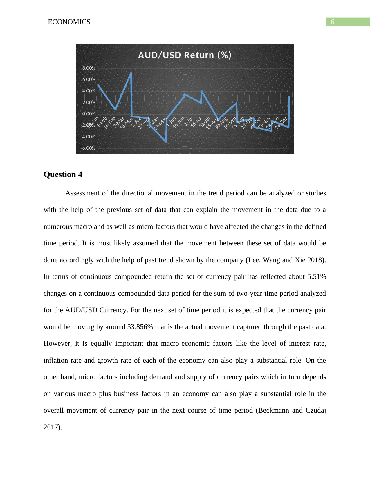
Question 5
The volatility assessment of Bitcoin would be done for a period of two-year of time
frame whereby the given set of data records has been analyzed for a sum of two-period. The
asset class selected for the purpose of analysis is definitely varied as Bitcoin as an asset class is a
digital crypto-currency that does not have any underlying asset making the prices of the assets to
be more volatile. In the given set of data period analyzed it was found that the values of crypto-
currency has varied significantly and the same could be well explained with the pattern formed
by the data analyzed (Indexmundi.com 2019).
16-Jan
31-Jan
15-Feb
2-Mar
17-Mar
1-Apr
16-Apr
1-May
16-May
31-May
15-Jun
30-Jun
15-Jul
30-Jul
14-Aug
29-Aug
13-Sep
28-Sep
13-Oct
28-Oct
12-Nov
27-Nov
12-Dec
-20.00%
-10.00%
0.00%
10.00%
20.00%
30.00%
40.00%
50.00%
60.00%
70.00%
BTC/USD Bitf inex Data
Question 6
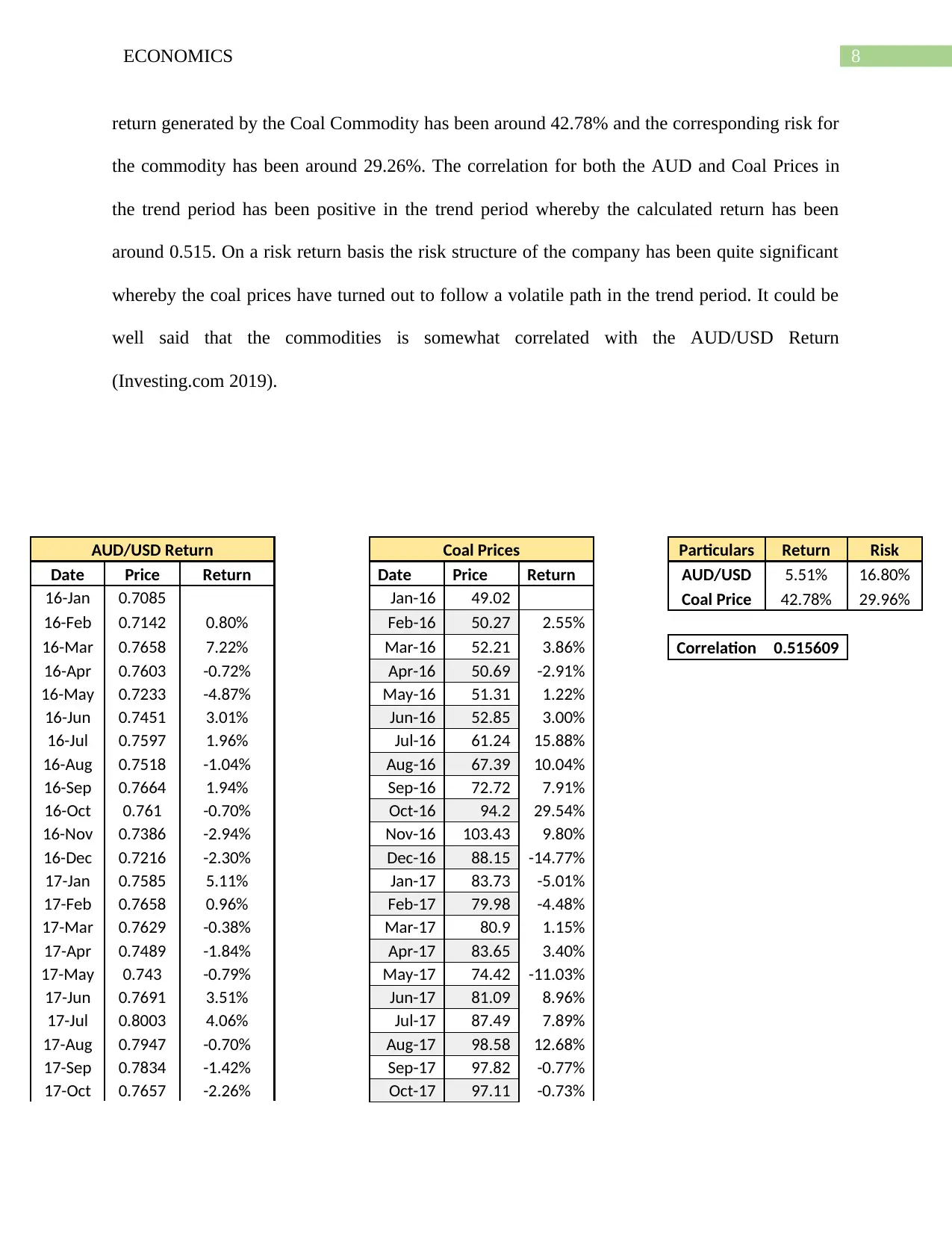
The association (correlation evident) between the AUD and the resultant value of Coal
Prices can be well compatible and researched based on the two-year data period analyzed. The
value of bulk minerals considered here is the prices of Coal that has been considered for the
purpose of analysis. The prices of Coal would be matched in accordance with the AUD/USD
Return for the trend period that would be analyzed for the company (Investing.com 2019). The

8ECONOMICS
return generated by the Coal Commodity has been around 42.78% and the corresponding risk for
the commodity has been around 29.26%. The correlation for both the AUD and Coal Prices in
the trend period has been positive in the trend period whereby the calculated return has been
around 0.515. On a risk return basis the risk structure of the company has been quite significant
whereby the coal prices have turned out to follow a volatile path in the trend period. It could be
well said that the commodities is somewhat correlated with the AUD/USD Return
(Investing.com 2019).
AUD/USD Return Coal Prices Particulars Return Risk
Date Price Return Date Price Return AUD/USD 5.51% 16.80%
16-Jan 0.7085 Jan-16 49.02 Coal Price 42.78% 29.96%
16-Feb 0.7142 0.80% Feb-16 50.27 2.55%
16-Mar 0.7658 7.22% Mar-16 52.21 3.86% Correlation 0.515609
16-Apr 0.7603 -0.72% Apr-16 50.69 -2.91%
16-May 0.7233 -4.87% May-16 51.31 1.22%
16-Jun 0.7451 3.01% Jun-16 52.85 3.00%
16-Jul 0.7597 1.96% Jul-16 61.24 15.88%
16-Aug 0.7518 -1.04% Aug-16 67.39 10.04%
16-Sep 0.7664 1.94% Sep-16 72.72 7.91%
16-Oct 0.761 -0.70% Oct-16 94.2 29.54%
16-Nov 0.7386 -2.94% Nov-16 103.43 9.80%
16-Dec 0.7216 -2.30% Dec-16 88.15 -14.77%
17-Jan 0.7585 5.11% Jan-17 83.73 -5.01%
17-Feb 0.7658 0.96% Feb-17 79.98 -4.48%
17-Mar 0.7629 -0.38% Mar-17 80.9 1.15%
17-Apr 0.7489 -1.84% Apr-17 83.65 3.40%
17-May 0.743 -0.79% May-17 74.42 -11.03%
17-Jun 0.7691 3.51% Jun-17 81.09 8.96%
17-Jul 0.8003 4.06% Jul-17 87.49 7.89%
17-Aug 0.7947 -0.70% Aug-17 98.58 12.68%
17-Sep 0.7834 -1.42% Sep-17 97.82 -0.77%
17-Oct 0.7657 -2.26% Oct-17 97.11 -0.73%

9ECONOMICS
17-Nov 0.7567 -1.18% Nov-17 96.64 -0.48%
17-Dec 0.7802 3.11% Dec-17 100.81 4.31%
The commodity currency name is given to some currencies whereby the same moves
with the world prices of commodity product as the country is heavily dependent on the export
and changes associated with these minerals taken into consideration. Commodities currencies are
also seen in developed economies as well like Canada and Australia. Due to the nature and effect
of the commodity currencies that are directly correlated to the value of the currency the same can
be problematic as well as an advantage to the economy. If the exports falls or rises the same
would be resulting to deflation or inflation on a respective basis. The impact of the same can be
more high when the value of currency is closely tied with the small set of commodities.
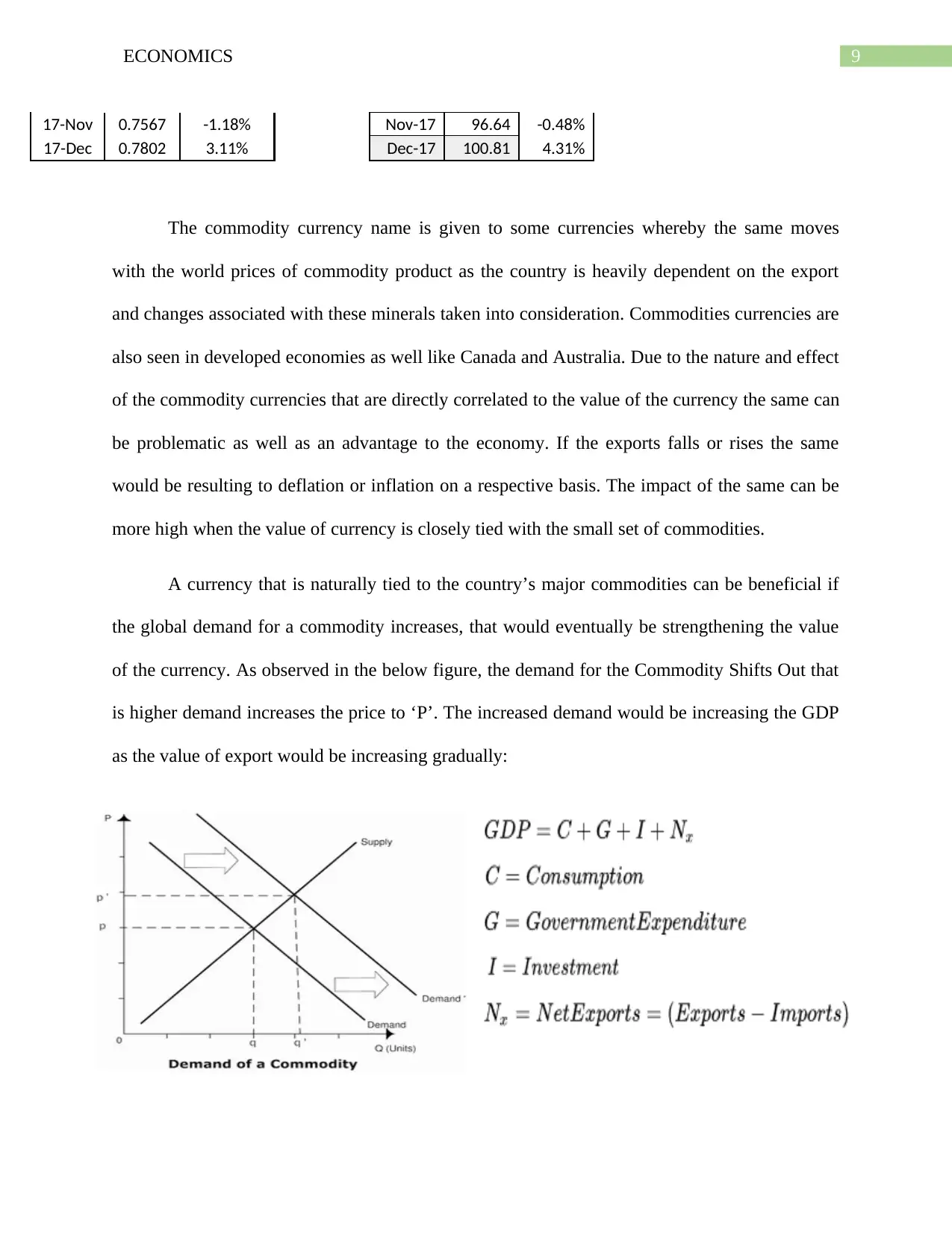
A currency that is naturally tied to the country’s major commodities can be beneficial if
the global demand for a commodity increases, that would eventually be strengthening the value
of the currency. As observed in the below figure, the demand for the Commodity Shifts Out that
is higher demand increases the price to ‘P’. The increased demand would be increasing the GDP
as the value of export would be increasing gradually:

10ECONOMICS

11ECONOMICS
References
Beckmann, J. and Czudaj, R., 2017. Exchange rate expectations since the financial crisis:
Performance evaluation and the role of monetary policy and safe haven. Journal of International
Money and Finance, 74, pp.283-300.
Guirguis, M., 2018. Application of a Log Likelihood Object In GARCH with T-distributed errors
and EGARCH With Generalised Error Distribution Model of the Spot AUD/USD Exchange Rate
Volatility. USD Exchange Rate Volatility.(September 21, 2018).
Hamilton, A., 2018. Understanding Exchange Rates and Why They Are Important| Bulletin–
December Quarter 2018. Bulletin, (December).
Indexmundi.com. (2019). Coal, Australian thermal coal - Monthly Price - Commodity Prices -
Price Charts, Data, and News - IndexMundi . [online] Available at:
https://www.indexmundi.com/commodities/?commodity=coal-australian&months=60 [Accessed
3 Aug. 2019].
Investing.com. 2019. AUD USD Historical Data - Investing.com. [online] Available at:
https://in.investing.com/currencies/aud-usd-historical-data [Accessed 2 Aug. 2019].
Investing.com. 2019. Gold Futures Historical Prices - Investing.com. [online] Available at:
https://in.investing.com/commodities/gold-historical-data [Accessed 3 Aug. 2019].
Ishizaki, R. and Inoue, M., 2018. Time-series analysis of multiple foreign exchange rates using
time-dependent pattern entropy. Physica A: Statistical Mechanics and its Applications, 490,
pp.967-974.