Economics Question 2022
VerifiedAdded on 2022/10/04
|17
|3216
|33
AI Summary
Contribute Materials
Your contribution can guide someone’s learning journey. Share your
documents today.

Economics
August 12
2019
August 12
2019
Secure Best Marks with AI Grader
Need help grading? Try our AI Grader for instant feedback on your assignments.
Table of Contents
Question 1: Production Possibility Curve..............................................................................................2
(1) Study of Joan’s Production Possibility Curve........................................................................2
(i) Production Possibility Curve for Joan....................................................................................2
(ii) Production Possibility Curve if opportunity cost was constant..........................................3
(iii) Combinations inside the Production Possibility Curve (PPC)............................................4
(iv) Combinations outside the Production Possibility Curve (PPC)..........................................5
(2) Concept of ‘Scarcity’.............................................................................................................6
Question 2: Demand and Supply...........................................................................................................7
(1) Improvement in technology...................................................................................................7
(i) Effect on the equilibrium price and quantity of solar-powered motor vehicle.......................7
(ii) Effect on the equilibrium price and quantity of conventional motor vehicle......................7
(2) Impact of the price ceiling.....................................................................................................7
Question 3: Price Elasticity of Demand.................................................................................................8
(1) Calculation of price elasticity using the midpoint method.....................................................8
(2) Price elasticity of demand for ice-creams in winter...............................................................9
(3) Price elasticity of demand for cigarettes..............................................................................10
Question 4: Types of Costs..................................................................................................................10
(1) Calculation of costs and profit.............................................................................................10
(2) Firm’s operation in short-run...............................................................................................11
(3) Price-taking firm profit maximization..................................................................................11

Question 5: Market Structure...............................................................................................................12
References...........................................................................................................................................14
References...........................................................................................................................................14
Question 1: Production Possibility Curve
(1) Study of Joan’s Production Possibility Curve
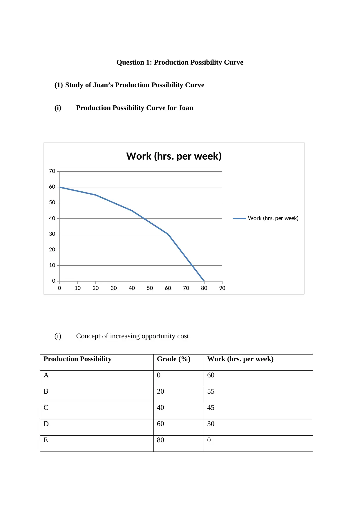
(i) Production Possibility Curve for Joan
0 10 20 30 40 50 60 70 80 90
0
10
20
30
40
50
60
70
Work (hrs. per week)
Work (hrs. per week)
(i) Concept of increasing opportunity cost
Production Possibility Grade (%) Work (hrs. per week)
A 0 60
B 20 55
C 40 45
D 60 30
E 80 0
(1) Study of Joan’s Production Possibility Curve
(i) Production Possibility Curve for Joan
0 10 20 30 40 50 60 70 80 90
0
10
20
30
40
50
60
70
Work (hrs. per week)
Work (hrs. per week)
(i) Concept of increasing opportunity cost
Production Possibility Grade (%) Work (hrs. per week)
A 0 60
B 20 55
C 40 45
D 60 30
E 80 0
Secure Best Marks with AI Grader
Need help grading? Try our AI Grader for instant feedback on your assignments.
Opportunity cost is said to be the cost of doing one activity in terms of the benefits
forgone from other activity. It occurs because resources are limited in nature and few
activities could be carried out with limited resources. In the problem, Joan has limited
time which is considered her limited resources. She has the option of increasing the
number of working hours for earning money or she can invest the time in studying to
improve her grades.
The concept of increasing opportunity cost states that when the production possibility
is increased for one item or activity the opportunity cost of producing an additional item
will also increase (Lugert, Thaller, Tetens, Schulz, & Krieter, 2016). This happens
because for every other production possibility of one item the cost of another item will be
more for the producer. Here, if Joan increases her working hours then the cost of
decreasing grades will also increase for her. This is why; production possibility curve is
used to determine all the possible combination of the activities or items that can be
carried on with the limited resources available with the producer.
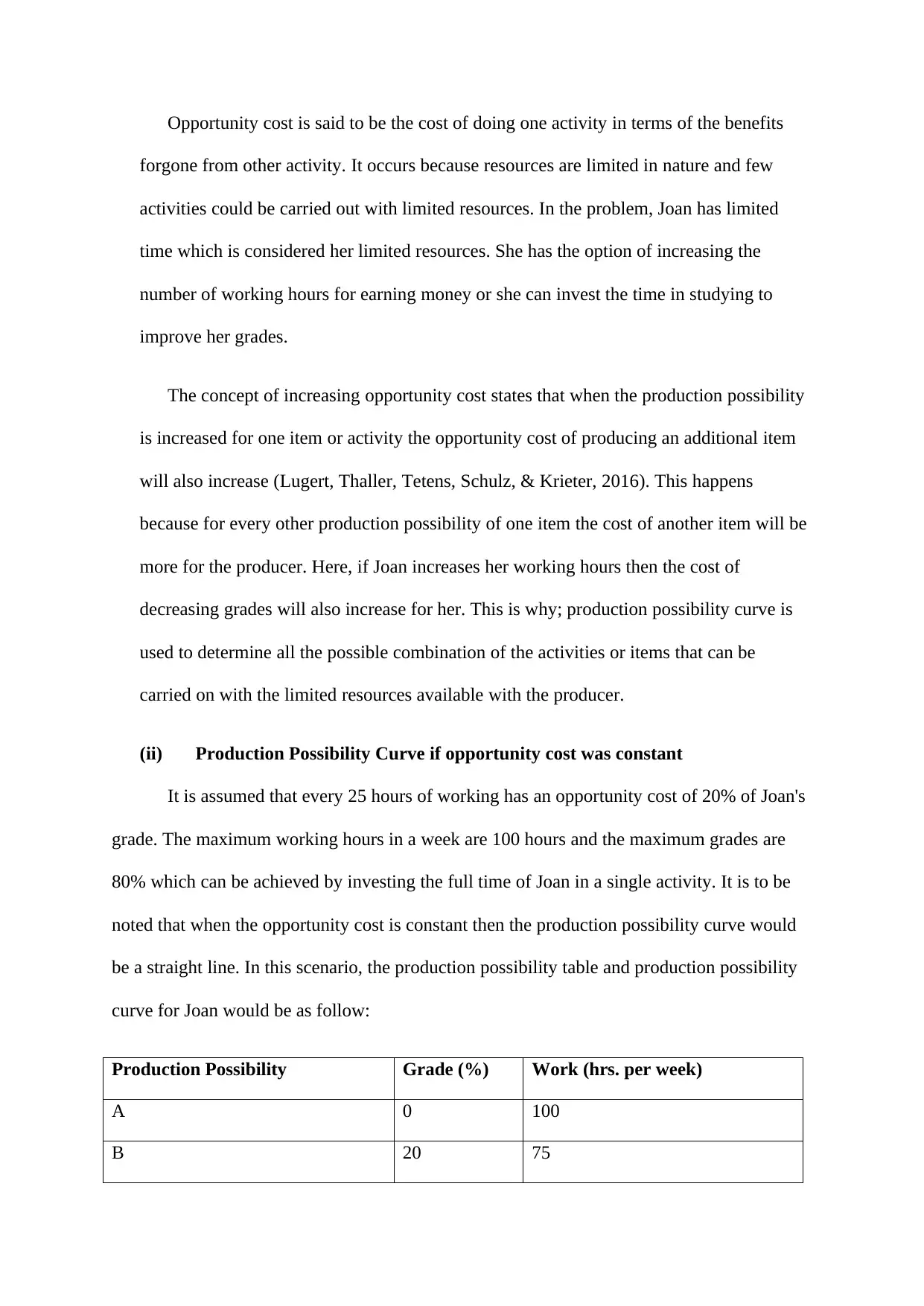
(ii) Production Possibility Curve if opportunity cost was constant
It is assumed that every 25 hours of working has an opportunity cost of 20% of Joan's
grade. The maximum working hours in a week are 100 hours and the maximum grades are
80% which can be achieved by investing the full time of Joan in a single activity. It is to be
noted that when the opportunity cost is constant then the production possibility curve would
be a straight line. In this scenario, the production possibility table and production possibility
curve for Joan would be as follow:
Production Possibility Grade (%) Work (hrs. per week)
A 0 100
B 20 75
forgone from other activity. It occurs because resources are limited in nature and few
activities could be carried out with limited resources. In the problem, Joan has limited
time which is considered her limited resources. She has the option of increasing the
number of working hours for earning money or she can invest the time in studying to
improve her grades.
The concept of increasing opportunity cost states that when the production possibility
is increased for one item or activity the opportunity cost of producing an additional item
will also increase (Lugert, Thaller, Tetens, Schulz, & Krieter, 2016). This happens
because for every other production possibility of one item the cost of another item will be
more for the producer. Here, if Joan increases her working hours then the cost of
decreasing grades will also increase for her. This is why; production possibility curve is
used to determine all the possible combination of the activities or items that can be
carried on with the limited resources available with the producer.
(ii) Production Possibility Curve if opportunity cost was constant
It is assumed that every 25 hours of working has an opportunity cost of 20% of Joan's
grade. The maximum working hours in a week are 100 hours and the maximum grades are
80% which can be achieved by investing the full time of Joan in a single activity. It is to be
noted that when the opportunity cost is constant then the production possibility curve would
be a straight line. In this scenario, the production possibility table and production possibility
curve for Joan would be as follow:
Production Possibility Grade (%) Work (hrs. per week)
A 0 100
B 20 75
C 40 50
D 60 25
E 80 0
0 10 20 30 40 50 60 70 80 90
0
20
40
60
80
100
120
Work (hrs. per week)
Work (hrs. per week)
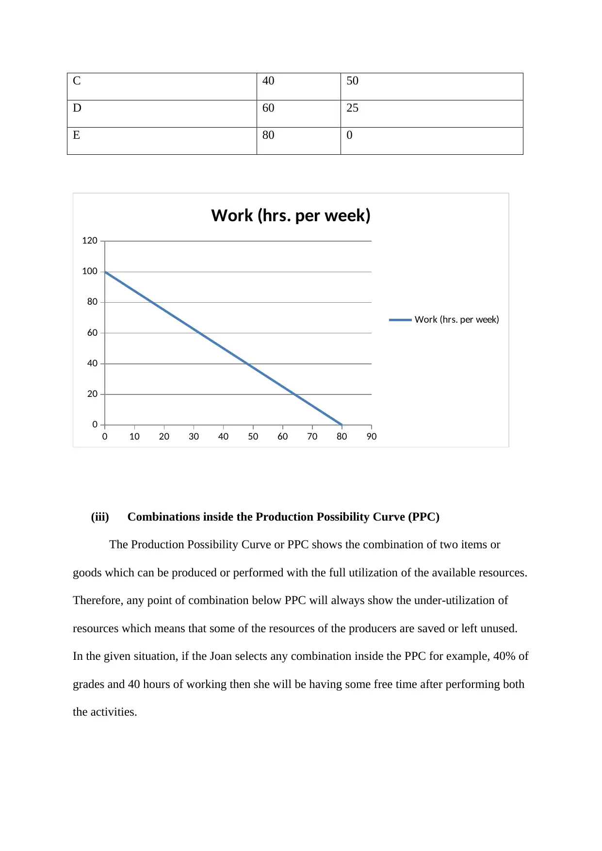
(iii) Combinations inside the Production Possibility Curve (PPC)
The Production Possibility Curve or PPC shows the combination of two items or
goods which can be produced or performed with the full utilization of the available resources.
Therefore, any point of combination below PPC will always show the under-utilization of
resources which means that some of the resources of the producers are saved or left unused.
In the given situation, if the Joan selects any combination inside the PPC for example, 40% of
grades and 40 hours of working then she will be having some free time after performing both
the activities.
D 60 25
E 80 0
0 10 20 30 40 50 60 70 80 90
0
20
40
60
80
100
120
Work (hrs. per week)
Work (hrs. per week)
(iii) Combinations inside the Production Possibility Curve (PPC)
The Production Possibility Curve or PPC shows the combination of two items or
goods which can be produced or performed with the full utilization of the available resources.
Therefore, any point of combination below PPC will always show the under-utilization of
resources which means that some of the resources of the producers are saved or left unused.
In the given situation, if the Joan selects any combination inside the PPC for example, 40% of
grades and 40 hours of working then she will be having some free time after performing both
the activities.
0 10 20 30 40 50 60 70 80 90
0
10
20
30
40
50
60
70
Work (hrs. per week)
Work (hrs. per week)
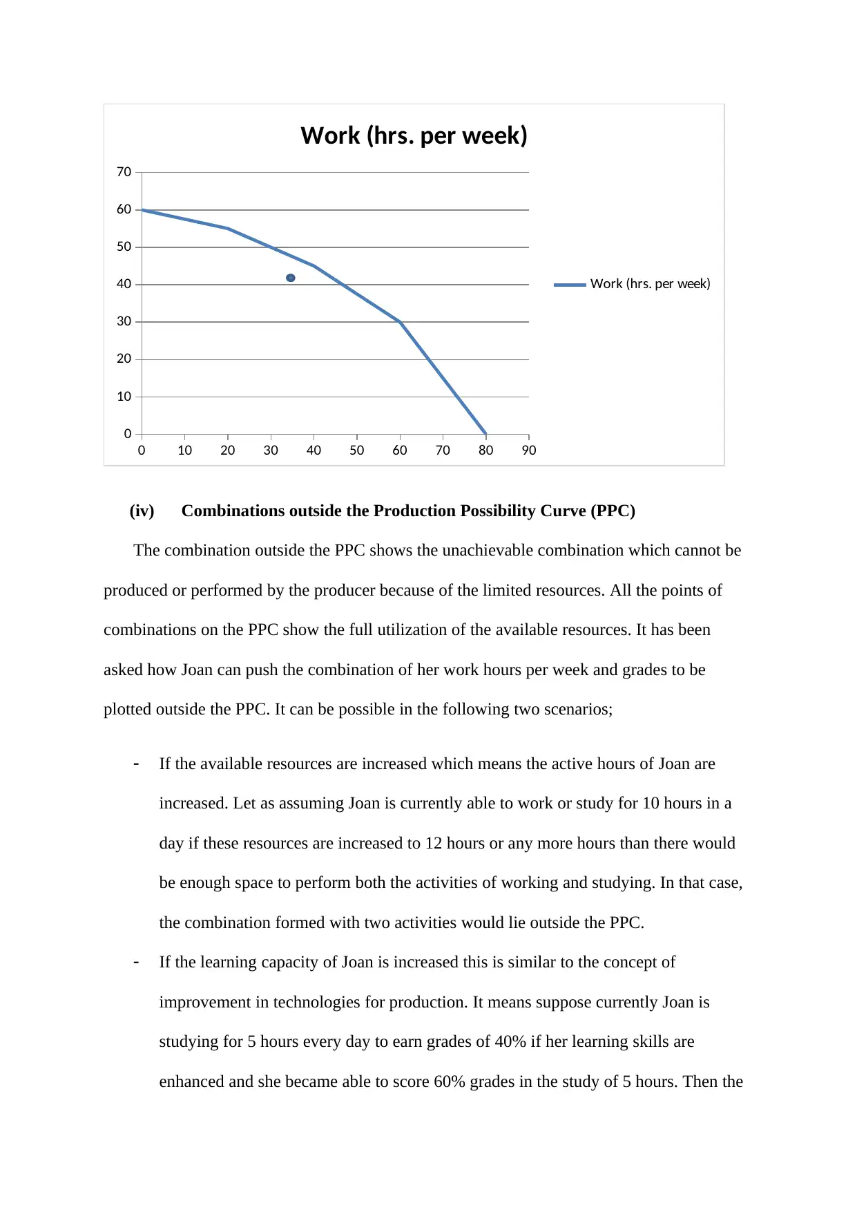
(iv) Combinations outside the Production Possibility Curve (PPC)
The combination outside the PPC shows the unachievable combination which cannot be
produced or performed by the producer because of the limited resources. All the points of
combinations on the PPC show the full utilization of the available resources. It has been
asked how Joan can push the combination of her work hours per week and grades to be
plotted outside the PPC. It can be possible in the following two scenarios;
If the available resources are increased which means the active hours of Joan are
increased. Let as assuming Joan is currently able to work or study for 10 hours in a
day if these resources are increased to 12 hours or any more hours than there would
be enough space to perform both the activities of working and studying. In that case,
the combination formed with two activities would lie outside the PPC.
If the learning capacity of Joan is increased this is similar to the concept of
improvement in technologies for production. It means suppose currently Joan is
studying for 5 hours every day to earn grades of 40% if her learning skills are
enhanced and she became able to score 60% grades in the study of 5 hours. Then the
0
10
20
30
40
50
60
70
Work (hrs. per week)
Work (hrs. per week)
(iv) Combinations outside the Production Possibility Curve (PPC)
The combination outside the PPC shows the unachievable combination which cannot be
produced or performed by the producer because of the limited resources. All the points of
combinations on the PPC show the full utilization of the available resources. It has been
asked how Joan can push the combination of her work hours per week and grades to be
plotted outside the PPC. It can be possible in the following two scenarios;
If the available resources are increased which means the active hours of Joan are
increased. Let as assuming Joan is currently able to work or study for 10 hours in a
day if these resources are increased to 12 hours or any more hours than there would
be enough space to perform both the activities of working and studying. In that case,
the combination formed with two activities would lie outside the PPC.
If the learning capacity of Joan is increased this is similar to the concept of
improvement in technologies for production. It means suppose currently Joan is
studying for 5 hours every day to earn grades of 40% if her learning skills are
enhanced and she became able to score 60% grades in the study of 5 hours. Then the
Paraphrase This Document
Need a fresh take? Get an instant paraphrase of this document with our AI Paraphraser
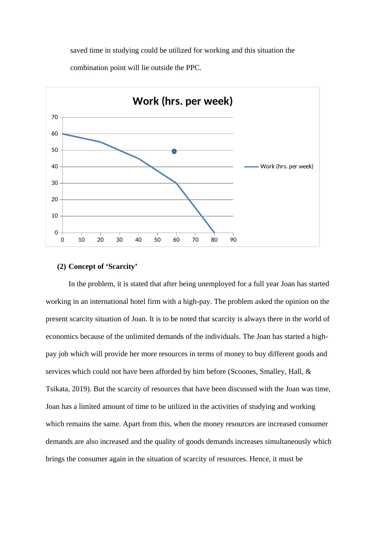
saved time in studying could be utilized for working and this situation the
combination point will lie outside the PPC.
0 10 20 30 40 50 60 70 80 90
0
10
20
30
40
50
60
70
Work (hrs. per week)
Work (hrs. per week)
(2) Concept of ‘Scarcity’
In the problem, it is stated that after being unemployed for a full year Joan has started
working in an international hotel firm with a high-pay. The problem asked the opinion on the
present scarcity situation of Joan. It is to be noted that scarcity is always there in the world of
economics because of the unlimited demands of the individuals. The Joan has started a high-
pay job which will provide her more resources in terms of money to buy different goods and
services which could not have been afforded by him before (Scoones, Smalley, Hall, &
Tsikata, 2019). But the scarcity of resources that have been discussed with the Joan was time,
Joan has a limited amount of time to be utilized in the activities of studying and working
which remains the same. Apart from this, when the money resources are increased consumer
demands are also increased and the quality of goods demands increases simultaneously which
brings the consumer again in the situation of scarcity of resources. Hence, it must be
understood that Joan can increase her standard of living or can buy more goods than before
but the problem of scarcity will always be there in the economic world.
Question 2: Demand and Supply
(1) Improvement in technology
(i) Effect on the equilibrium price and quantity of solar-powered motor vehicle
The improvement in the manufacturing technology of the solar power motor vehicle
will reduce the cost of production of these vehicles. The reduction in the production cost will
reduce the selling price of the item which will impact the demand for the product (Igos,
Rugani, Rege, Benetto, Drouet, & Zachary, 2015). The law of demand states that when the
price of the good is decreased its demanded quantity will increase. Hence, the equilibrium
price of the vehicle will decrease and the equilibrium quantity will increase.
(ii) Effect on the equilibrium price and quantity of conventional motor vehicle
It is a problem related to the impact on the substitute goods. The conventional motor
vehicle can be used in place of solar motor vehicles. When the price of substitute goods
decreases the demand for the original goods also decreases because the consumers shift to
substitute goods. Here, the demand for the conventional motor vehicle will decrease and the
equilibrium price will adjust accordingly.
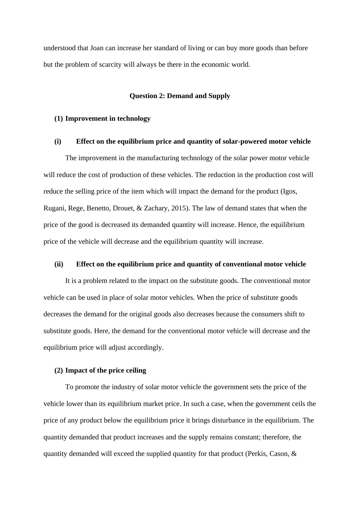
(2) Impact of the price ceiling
To promote the industry of solar motor vehicle the government sets the price of the
vehicle lower than its equilibrium market price. In such a case, when the government ceils the
price of any product below the equilibrium price it brings disturbance in the equilibrium. The
quantity demanded that product increases and the supply remains constant; therefore, the
quantity demanded will exceed the supplied quantity for that product (Perkis, Cason, &
but the problem of scarcity will always be there in the economic world.
Question 2: Demand and Supply
(1) Improvement in technology
(i) Effect on the equilibrium price and quantity of solar-powered motor vehicle
The improvement in the manufacturing technology of the solar power motor vehicle
will reduce the cost of production of these vehicles. The reduction in the production cost will
reduce the selling price of the item which will impact the demand for the product (Igos,
Rugani, Rege, Benetto, Drouet, & Zachary, 2015). The law of demand states that when the
price of the good is decreased its demanded quantity will increase. Hence, the equilibrium
price of the vehicle will decrease and the equilibrium quantity will increase.
(ii) Effect on the equilibrium price and quantity of conventional motor vehicle
It is a problem related to the impact on the substitute goods. The conventional motor
vehicle can be used in place of solar motor vehicles. When the price of substitute goods
decreases the demand for the original goods also decreases because the consumers shift to
substitute goods. Here, the demand for the conventional motor vehicle will decrease and the
equilibrium price will adjust accordingly.
(2) Impact of the price ceiling
To promote the industry of solar motor vehicle the government sets the price of the
vehicle lower than its equilibrium market price. In such a case, when the government ceils the
price of any product below the equilibrium price it brings disturbance in the equilibrium. The
quantity demanded that product increases and the supply remains constant; therefore, the
quantity demanded will exceed the supplied quantity for that product (Perkis, Cason, &
Tyner, 2016). However, the government agenda is partially completed with this method as it
increased the number of consumers in the solar vehicle industry.
150 200 250 300 350
0
10
20
30
40
50
60
Demand
Supply
EQ
EP
In the graph, the red line shows supply and the blue line shows the demand. The price
ceiling by the government is denoted by the green line in parallel to the X-axis. The blue dot
shows the new intersection point of demand and price.
Question 3: Price Elasticity of Demand
(1) Calculation of price elasticity using the midpoint method
Price elasticity of demand shows the percentage change in the quantity demanded of a
product due to a change in its price (Miller, & Alberini, 2016).
To calculate the price elasticity of demand with the midpoint method first we have to
calculate the percentage change in the quantity and price of the product, here ice-cream.
% change in Price = (P2-P1)/ {(P2+P1)/ 2}
% change in Quantity = (Q2-Q1)/ {(Q2+Q1)/ 2}
Secure Best Marks with AI Grader
Need help grading? Try our AI Grader for instant feedback on your assignments.
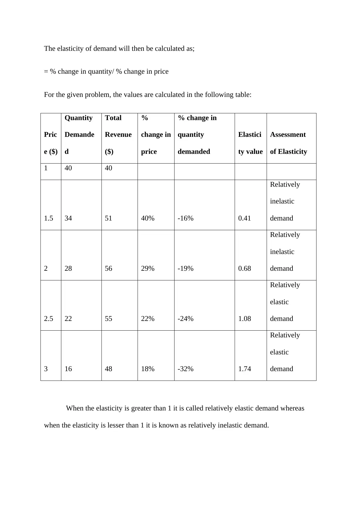
The elasticity of demand will then be calculated as;
= % change in quantity/ % change in price
For the given problem, the values are calculated in the following table:
Pric
e ($)
Quantity
Demande
d
Total
Revenue
($)
%
change in
price
% change in
quantity
demanded
Elastici
ty value
Assessment
of Elasticity
1 40 40
1.5 34 51 40% -16% 0.41
Relatively
inelastic
demand
2 28 56 29% -19% 0.68
Relatively
inelastic
demand
2.5 22 55 22% -24% 1.08
Relatively
elastic
demand
3 16 48 18% -32% 1.74
Relatively
elastic
demand
When the elasticity is greater than 1 it is called relatively elastic demand whereas
when the elasticity is lesser than 1 it is known as relatively inelastic demand.
(2) Price elasticity of demand for ice-creams in winter
The price elasticity of demand for the ice-creams will be relatively inelastic in winter
because in the winter the weather is already very cool and in such weather the demand for
ice-cream is low. However, the ice-creams are sold in winter in low quantity and such
demand will not be much affected by the changes in prices as seen in the summers.
Therefore, the demand will be relatively inelastic in winters.
(3) Price elasticity of demand for cigarettes
Cigarettes are the items that are put in the categories of addictive items and the
elasticity of such items are assumed to be inelastic or relatively inelastic (Jawad, Lee, Glantz,
& Millett, 2018). The tobacco products are assumed to have an elasticity of demand lesser
than one or inelastic which its demand will have a little or no impact on the price change of
the items.
Question 4: Types of Costs
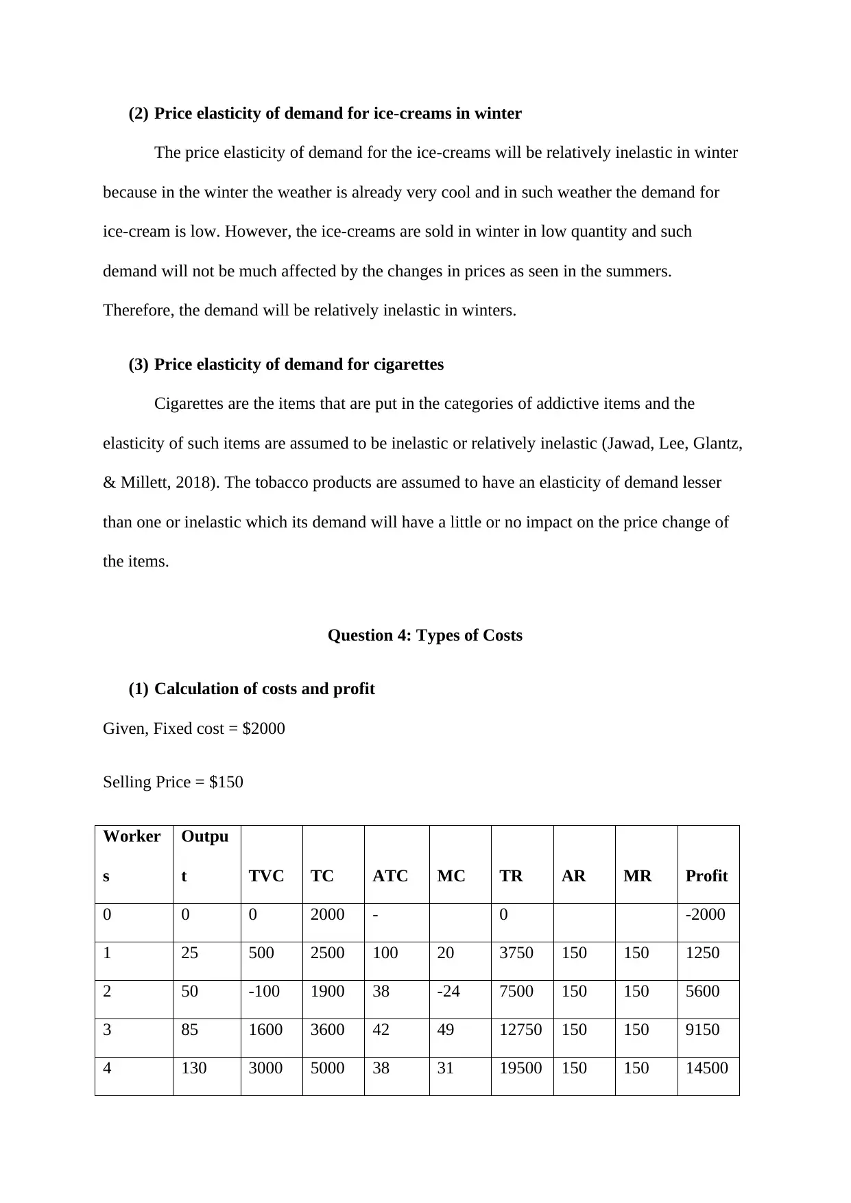
(1) Calculation of costs and profit
Given, Fixed cost = $2000
Selling Price = $150
Worker
s
Outpu
t TVC TC ATC MC TR AR MR Profit
0 0 0 2000 - 0 -2000
1 25 500 2500 100 20 3750 150 150 1250
2 50 -100 1900 38 -24 7500 150 150 5600
3 85 1600 3600 42 49 12750 150 150 9150
4 130 3000 5000 38 31 19500 150 150 14500
The price elasticity of demand for the ice-creams will be relatively inelastic in winter
because in the winter the weather is already very cool and in such weather the demand for
ice-cream is low. However, the ice-creams are sold in winter in low quantity and such
demand will not be much affected by the changes in prices as seen in the summers.
Therefore, the demand will be relatively inelastic in winters.
(3) Price elasticity of demand for cigarettes
Cigarettes are the items that are put in the categories of addictive items and the
elasticity of such items are assumed to be inelastic or relatively inelastic (Jawad, Lee, Glantz,
& Millett, 2018). The tobacco products are assumed to have an elasticity of demand lesser
than one or inelastic which its demand will have a little or no impact on the price change of
the items.
Question 4: Types of Costs
(1) Calculation of costs and profit
Given, Fixed cost = $2000
Selling Price = $150
Worker
s
Outpu
t TVC TC ATC MC TR AR MR Profit
0 0 0 2000 - 0 -2000
1 25 500 2500 100 20 3750 150 150 1250
2 50 -100 1900 38 -24 7500 150 150 5600
3 85 1600 3600 42 49 12750 150 150 9150
4 130 3000 5000 38 31 19500 150 150 14500
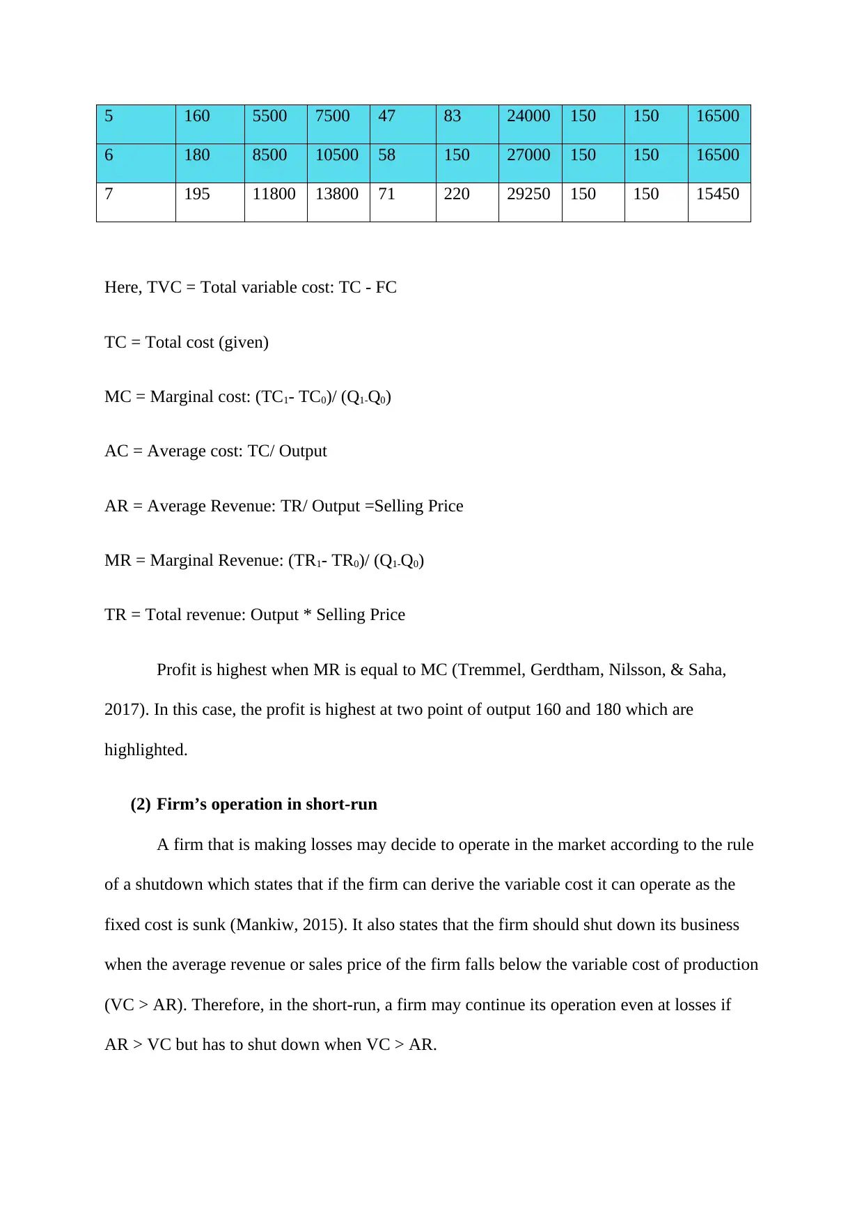
5 160 5500 7500 47 83 24000 150 150 16500
6 180 8500 10500 58 150 27000 150 150 16500
7 195 11800 13800 71 220 29250 150 150 15450
Here, TVC = Total variable cost: TC - FC
TC = Total cost (given)
MC = Marginal cost: (TC1- TC0)/ (Q1-Q0)
AC = Average cost: TC/ Output
AR = Average Revenue: TR/ Output =Selling Price
MR = Marginal Revenue: (TR1- TR0)/ (Q1-Q0)
TR = Total revenue: Output * Selling Price
Profit is highest when MR is equal to MC (Tremmel, Gerdtham, Nilsson, & Saha,
2017). In this case, the profit is highest at two point of output 160 and 180 which are
highlighted.
(2) Firm’s operation in short-run
A firm that is making losses may decide to operate in the market according to the rule
of a shutdown which states that if the firm can derive the variable cost it can operate as the
fixed cost is sunk (Mankiw, 2015). It also states that the firm should shut down its business
when the average revenue or sales price of the firm falls below the variable cost of production
(VC > AR). Therefore, in the short-run, a firm may continue its operation even at losses if
AR > VC but has to shut down when VC > AR.
Paraphrase This Document
Need a fresh take? Get an instant paraphrase of this document with our AI Paraphraser
(3) Price-taking firm profit maximization
A price-taking firm is the one which has to accept the market price as its selling price
while operating in the market. These firms determine their profit maximization by the firm's
optimal output rule (Wong, 2015). This rule states that the firm will earn a maximum profit
when the marginal cost of the goods is equal to the market price of the product. Hence profit
is maximized when AR= MC or MC =MR.
Question 5: Market Structure
A Monopoly market structure is the market structure in which there is a single seller
of the product who has full control over the prices of the product because of high demand
(Weller, Kleer, & Piller, 2015). On the other hand, the perfect competition market is the one
where there is a large number of sellers and buyers (Simatele, 2015). In the perfect
competition market, the seller is a price taker from the market and not the price maker.
The Australian banking industry is operating in an Oligopoly market structure where
there are very few large firms that collectively excise control on the market share. The
Australian banking industry is said to be closer to the monopoly market because monopoly
comes into existence when there is a low number of sellers or producers. This happens
because of the restrictions on the entry of new firms in the industry. The banking industry is a
type of industry that requires a huge investment to begin. The Australian banking industry
presently has very few numbers of banks (Sheedy, & Griffin, 2018). Also, the restrictions on
the entry of the because of large investment pushes the industry to the monopoly structure.
It is understood that the customers are always benefitted in the perfect competition
market as in this market the prices are fixed with the market demand and supply equilibrium
and the firms have to accept the market price as selling price of their product. However, in
the monopoly market structure, the firm is the price maker and it sells is goods or services at

the prices which are beneficial to their business. In such a situation, the inclination of the
banking industry towards the monopoly structure is against the public interest.
Apart from this banking industry, the Australian post already holds the monopoly in
the market of Australia.
banking industry towards the monopoly structure is against the public interest.
Apart from this banking industry, the Australian post already holds the monopoly in
the market of Australia.

References
Igos, E., Rugani, B., Rege, S., Benetto, E., Drouet, L., & Zachary, D. S. (2015). Combination
of equilibrium models and hybrid life cycle-input–output analysis to predict the
environmental impacts of energy policy scenarios. Applied energy, 145, 234-245.
Jawad, M., Lee, J. T., Glantz, S., & Millett, C. (2018). Price elasticity of demand of non-
cigarette tobacco products: a systematic review and meta-analysis. Tobacco
control, 27(6), 689-695.
Lugert, V., Thaller, G., Tetens, J., Schulz, C., & Krieter, J. (2016). A review on fish growth
calculation: multiple functions in fish production and their specific
application. Reviews in Aquaculture, 8(1), 30-42.
Mankiw, N. G. (2015). Firms in competitive markets. Principles of economics, 279-298.).
Firms in competitive markets. Principles of economics, 279-298.
Miller, M., & Alberini, A. (2016). Sensitivity of price elasticity of demand to aggregation,
unobserved heterogeneity, price trends, and price endogeneity: Evidence from US
Data. Energy Policy, 97, 235-249.
Perkis, D. F., Cason, T. N., & Tyner, W. E. (2016). An experimental investigation of hard
and soft price ceilings in emissions permit markets. Environmental and Resource
Economics, 63(4), 703-718.
Scoones, I., Smalley, R., Hall, R., & Tsikata, D. (2019). Narratives of scarcity: Framing the
global land rush. Geoforum, 101, 231-241.
Sheedy, E., & Griffin, B. (2018). Risk governance, structures, culture, and behavior: A view
from the inside. Corporate Governance: An International Review, 26(1), 4-22.
Secure Best Marks with AI Grader
Need help grading? Try our AI Grader for instant feedback on your assignments.
Simatele, M. (2015). Market Structure and competition in the South African banking
sector. Procedia Economics and Finance, 30, 825-835.
Tremmel, M., Gerdtham, U. G., Nilsson, P., & Saha, S. (2017). Economic burden of obesity:
a systematic literature review. International journal of environmental research and
public health, 14(4), 435.
Weller, C., Kleer, R., & Piller, F. T. (2015). Economic implications of 3D printing: Market
structure models in light of additive manufacturing revisited. International Journal of
Production Economics, 164, 43-56.
Wong, K. P. (2015). A smooth ambiguity model of the competitive firm. Bulletin of
Economic Research, 67(S1), S97-S110.
1 out of 17
Related Documents


Your All-in-One AI-Powered Toolkit for Academic Success.
+13062052269
info@desklib.com
Available 24*7 on WhatsApp / Email
![[object Object]](/_next/static/media/star-bottom.7253800d.svg)
Unlock your academic potential
© 2024 | Zucol Services PVT LTD | All rights reserved.