Economics and Quantitative Analysis Assignment

This assignment covers topics like ecological footprint, population growth, harvesting of fish, and more. It provides information on the sustainability of human reliance on natural resources, knife edge equilibrium, and the effect of density on population growth. The document type is an Economics assignment and the course code is 11. The course name, college/university, and assignment type are not mentioned.

ECONOMICS ASSIGNMENT. 1
ECONOMICS AND QUANTITATIVE ANALYSIS.
Name:
Tutor:
Institution:
Course:
Date:

ECONOMICS ASSIGNMENT. 2
Economics and Quantitative Analysis.
Section A: Ecological Footprint.
a. From the graph, the human population is lived below earth’s natural bio capacity between
1961 to 1970; here human reliance on natural resources was lower than the ability of land
to generate renewable resources and clean its unwanted and it this reflects a sustainable
period, the year around 1971 the ecological footprints was equal to bio capacity which
means that the human reliance to natural resources was equal to its ability to generate
renewable resources and clean up its waste. Between 1972 and 2012 over 40 years there
has been greater human reliance on the natural resources than the ability of land to
generate renewable resources and clean up its unwanted. The Ecological footprints is
greater than the bio capacity. This situation is unsustainable because the human being
rely on the natural resources from the land that does not have the capability of
regenerating renewable resources and cleaning the unwanted elements thereby, resulting
to excess of ecological footprints than the bio capacity (Hussen, 2018).
b. From the graph, the human population is living below earth’s natural bio capacity. It
simply means that there is a lower human reliance on the natural resources than the
ability of land to generate renewable resources and clean up its unwanted. The Ecological
footprints is lower than the bio capacity (Luo, et al., 2018). This situation has been in
existence since 1961 and it is approximately 51 years. This situation is sustainable
because the capability of generating renewable resources and cleaning the waste is higher
than human being reliance on the natural resources from the land, resulting to excess of
bio capacity than the ecological footprints (Yang & Fan, 2019).
c. From the graph, the human population is living beyond earth’s natural bio capacity. It
simply means that there is a higher human reliance on the natural resources than the
ability of land to generate renewable resources and clean up its unwanted. The Ecological
footprints is greater than the bio capacity. This situation has been in existence since 1961
and it is approximately 51 years. This situation is unsustainable because the capability of
generating renewable resources and cleaning the waste is much slower as compared to
human being reliance on the natural resources from the land, resulting to excess of
ecological footprints than the bio capacity (Toth & Szigeti, 2016).

ECONOMICS ASSIGNMENT. 3
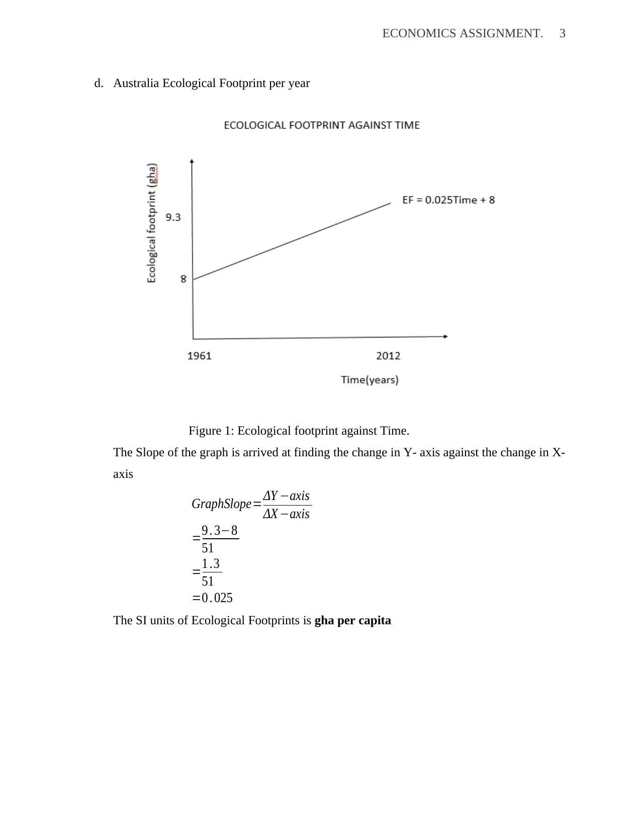
d. Australia Ecological Footprint per year
Figure 1: Ecological footprint against Time.
The Slope of the graph is arrived at finding the change in Y- axis against the change in X-
axis
GraphSlope=ΔY −axis
ΔX −axis
=9 . 3−8
51
=1 .3
51
=0 . 025
The SI units of Ecological Footprints is gha per capita

ECONOMICS ASSIGNMENT. 4
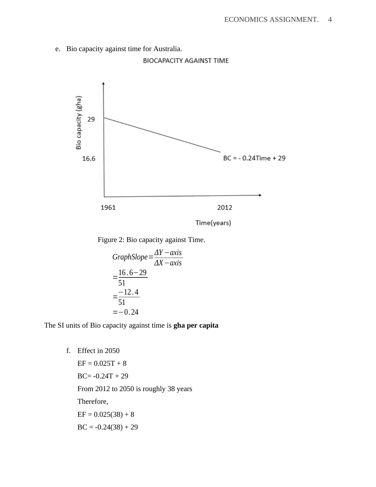
e. Bio capacity against time for Australia.
Figure 2: Bio capacity against Time.
GraphSlope=ΔY −axis
ΔX −axis
=16 . 6−29
51
=−12 . 4
51
=−0. 24
The SI units of Bio capacity against time is gha per capita
f. Effect in 2050
EF = 0.025T + 8
BC= -0.24T + 29
From 2012 to 2050 is roughly 38 years
Therefore,
EF = 0.025(38) + 8
BC = -0.24(38) + 29

ECONOMICS ASSIGNMENT. 5
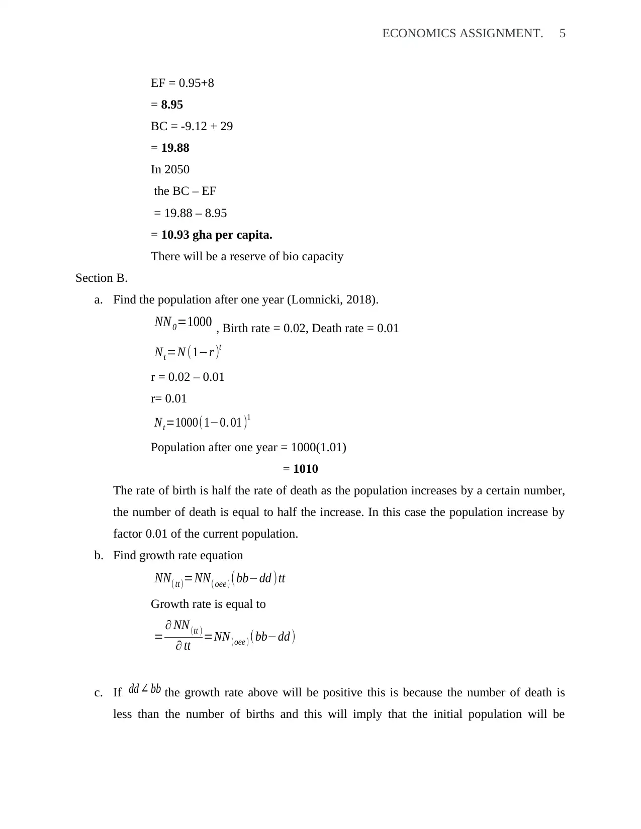
EF = 0.95+8
= 8.95
BC = -9.12 + 29
= 19.88
In 2050
the BC – EF
= 19.88 – 8.95
= 10.93 gha per capita.
There will be a reserve of bio capacity
Section B.
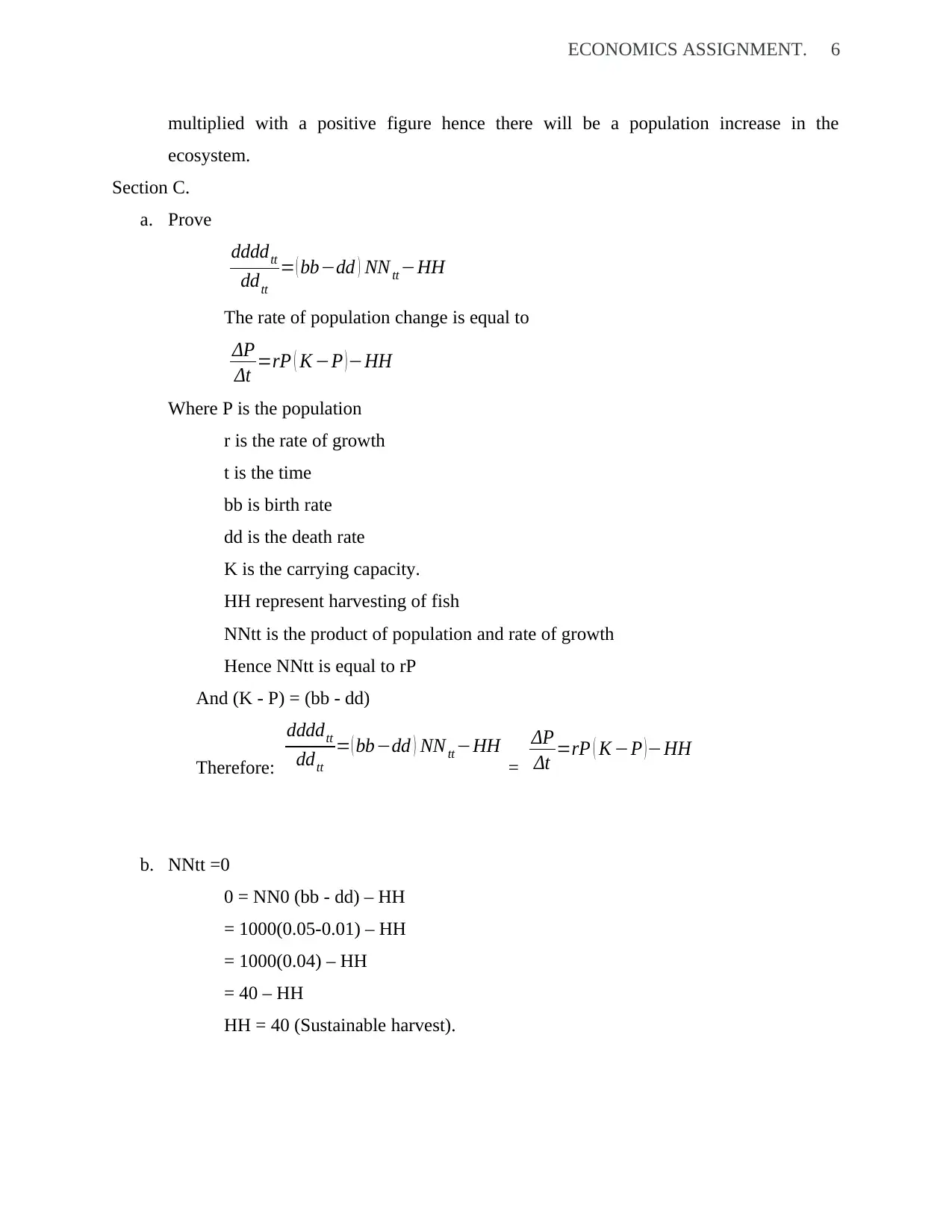
a. Find the population after one year (Lomnicki, 2018).
NN 0=1000 , Birth rate = 0.02, Death rate = 0.01
Nt=N (1−r )t
r = 0.02 – 0.01
r= 0.01
Nt=1000(1−0. 01 )1
Population after one year = 1000(1.01)
= 1010
The rate of birth is half the rate of death as the population increases by a certain number,
the number of death is equal to half the increase. In this case the population increase by
factor 0.01 of the current population.
b. Find growth rate equation
NN( tt)=NN( oee ) (bb−dd )tt
Growth rate is equal to
= ∂ NN (tt )
∂ tt =NN (oee ) (bb−dd )
c. If dd ∠ bb the growth rate above will be positive this is because the number of death is
less than the number of births and this will imply that the initial population will be

ECONOMICS ASSIGNMENT. 6
multiplied with a positive figure hence there will be a population increase in the
ecosystem.
Section C.
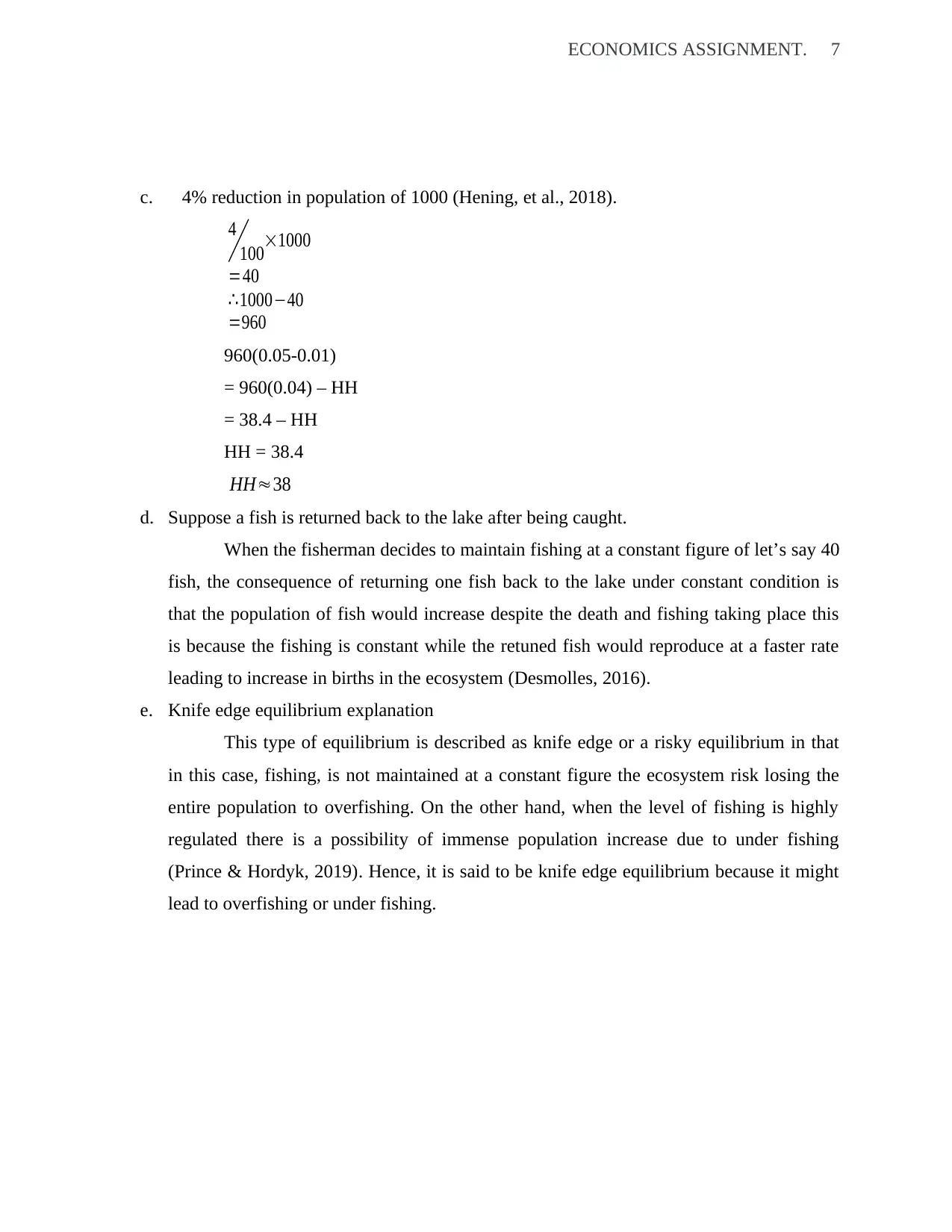
a. Prove
ddddtt
ddtt
= ( bb−dd ) NN tt −HH
The rate of population change is equal to
ΔP
Δt =rP ( K −P ) −HH
Where P is the population
r is the rate of growth
t is the time
bb is birth rate
dd is the death rate
K is the carrying capacity.
HH represent harvesting of fish
NNtt is the product of population and rate of growth
Hence NNtt is equal to rP
And (K - P) = (bb - dd)
Therefore:
ddddtt
ddtt
= ( bb−dd ) NN tt −HH
=
ΔP
Δt =rP ( K −P ) −HH
b. NNtt =0
0 = NN0 (bb - dd) – HH
= 1000(0.05-0.01) – HH
= 1000(0.04) – HH
= 40 – HH
HH = 40 (Sustainable harvest).

ECONOMICS ASSIGNMENT. 7
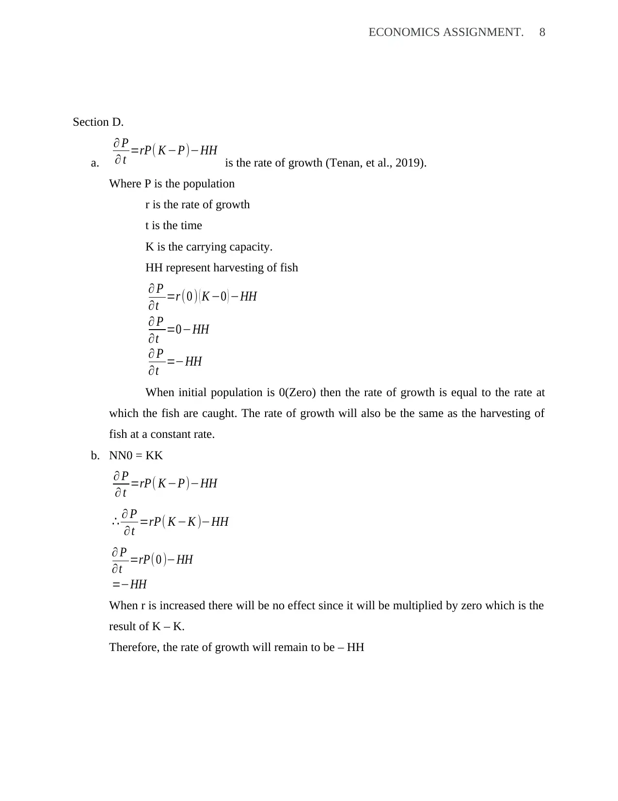
c. 4% reduction in population of 1000 (Hening, et al., 2018).
4
100×1000
=40
∴1000−40
=960
960(0.05-0.01)
= 960(0.04) – HH
= 38.4 – HH
HH = 38.4
HH≈38
d. Suppose a fish is returned back to the lake after being caught.
When the fisherman decides to maintain fishing at a constant figure of let’s say 40
fish, the consequence of returning one fish back to the lake under constant condition is
that the population of fish would increase despite the death and fishing taking place this
is because the fishing is constant while the retuned fish would reproduce at a faster rate
leading to increase in births in the ecosystem (Desmolles, 2016).
e. Knife edge equilibrium explanation
This type of equilibrium is described as knife edge or a risky equilibrium in that
in this case, fishing, is not maintained at a constant figure the ecosystem risk losing the
entire population to overfishing. On the other hand, when the level of fishing is highly
regulated there is a possibility of immense population increase due to under fishing
(Prince & Hordyk, 2019). Hence, it is said to be knife edge equilibrium because it might
lead to overfishing or under fishing.

ECONOMICS ASSIGNMENT. 8
Section D.
a.
∂ P
∂ t =rP( K −P)−HH is the rate of growth (Tenan, et al., 2019).
Where P is the population
r is the rate of growth
t is the time
K is the carrying capacity.
HH represent harvesting of fish
∂ P
∂t =r ( 0 ) ( K −0 ) −HH
∂ P
∂t =0−HH
∂ P
∂t =−HH
When initial population is 0(Zero) then the rate of growth is equal to the rate at
which the fish are caught. The rate of growth will also be the same as the harvesting of
fish at a constant rate.
b. NN0 = KK
∂ P
∂ t =rP( K −P)−HH
∴ ∂ P
∂t =rP( K −K )−HH
∂ P
∂t =rP(0 )−HH
=−HH
When r is increased there will be no effect since it will be multiplied by zero which is the
result of K – K.
Therefore, the rate of growth will remain to be – HH

ECONOMICS ASSIGNMENT. 9
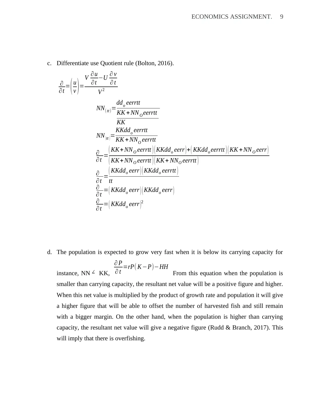
c. Differentiate use Quotient rule (Bolton, 2016).
∂
∂t = ( u
v ) =
V ∂ u
∂t −U ∂ v
∂ t
V 2
NN( tt)=ddo eerrtt
KK + NN O eerrtt
KK
NN ( tt ) =KKddo eerrtt
KK + NNO eerrtt
∂
∂t = ( KK+ NN O eerrtt ) ( KKddo eerr ) + ( KKddo eerrtt ) ( KK + NN O eerr )
( KK+ NN O eerrtt ) ( KK + NNO eerrtt )
∂
∂t = ( KKddo eerr ) ( KKddo eerrtt )
tt
∂
∂t = ( KKddo eerr ) ( KKddo eerr )
∂
∂t = ( KKddo eerr )
2
d. The population is expected to grow very fast when it is below its carrying capacity for
instance, NN ∠ KK,
∂ P
∂ t =rP( K −P)−HH From this equation when the population is
smaller than carrying capacity, the resultant net value will be a positive figure and higher.
When this net value is multiplied by the product of growth rate and population it will give
a higher figure that will be able to offset the number of harvested fish and still remain
with a bigger margin. On the other hand, when the population is higher than carrying
capacity, the resultant net value will give a negative figure (Rudd & Branch, 2017). This
will imply that there is overfishing.

ECONOMICS ASSIGNMENT. 10
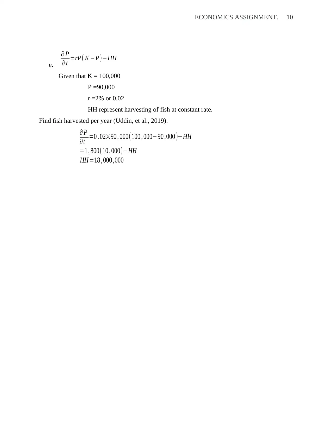
e.
∂ P
∂ t =rP( K −P)−HH
Given that K = 100,000
P =90,000
r =2% or 0.02
HH represent harvesting of fish at constant rate.
Find fish harvested per year (Uddin, et al., 2019).
∂ P
∂t =0 . 02×90 , 000(100 , 000−90 ,000 )−HH
=1 , 800(10 , 000)−HH
HH =18 , 000 ,000

ECONOMICS ASSIGNMENT. 11
Bibliography
Bolton, W., 2016. Differentiation and integration. s.l.:Routledge.
Desmolles, F., 2016. History of the Fish Fauna of Lake Pavin: A Population Heavily Influenced.
Lake Pavin: History, geology, biogeochemistry, and sedimentology of a deep meromictic maar
lake, pp. 345-349.
Hening, A., Nguyen, D., Ungureanu, S. & Wong, T., 2018. Asymptotic harvesting of populations
in random environments. Journal of mathematical biology, pp. 1-37.
Hussen, A., 2018. Principles of environmental economics and sustainability: an integrated
economic and ecological approach. s.l.:Routledge.
Lomnicki, A., 2018. Population ecology from the individual perspective. In Individual-based
models and approaches in ecology. s.l.:Chapman and Hall/CRC.
Luo, W. et al., 2018. Urbanization-induced ecological degradation in Midwestern China: An
analysis based on an improved ecological footprint model. Resources, Conservation and
Recycling, 137(2), pp. 113-125.
Prince, J. & Hordyk, A., 2019. What to do when you have almost nothing: A simple quantitative
prescription for managing extremely data‐poor fisheries. Fish and Fisheries, 20(2), pp. 224-238.
Rudd, M. & Branch, T., 2017. Does unreported catch lead to overfishing?. Fish and fisheries,
18(2), pp. 313-323.
Tenan, S., Tavecchia, G., Oro, D. & Pradel, R., 2019. Assessing the effect of density on
population growth when modeling individual encounter data. Ecology, 100(3), pp. e02595-
e02604.
Toth, G. & Szigeti, C., 2016. The historical ecological footprint: From over-population to over-
consumption. Ecological Indicators, 60(3), pp. 283-291.
Uddin, G., Alam, K. & Gow, J., 2019. Ecological and economic growth interdependency in the
Asian economies: an empirical analysis. Environmental Science and Pollution Research, pp. 1-
14.
Yang, Y. & Fan, M., 2019. Analysis of the spatial-temporal differences and fairness of the
regional energy ecological footprint of the Silk Road Economic Belt (China Section). Journal of
Cleaner Production, 215(3), pp. 1246-1261.

ECONOMICS ASSIGNMENT. 12