Economics Homework: GDP Calculation, Labor Demand, and Fiscal Policy

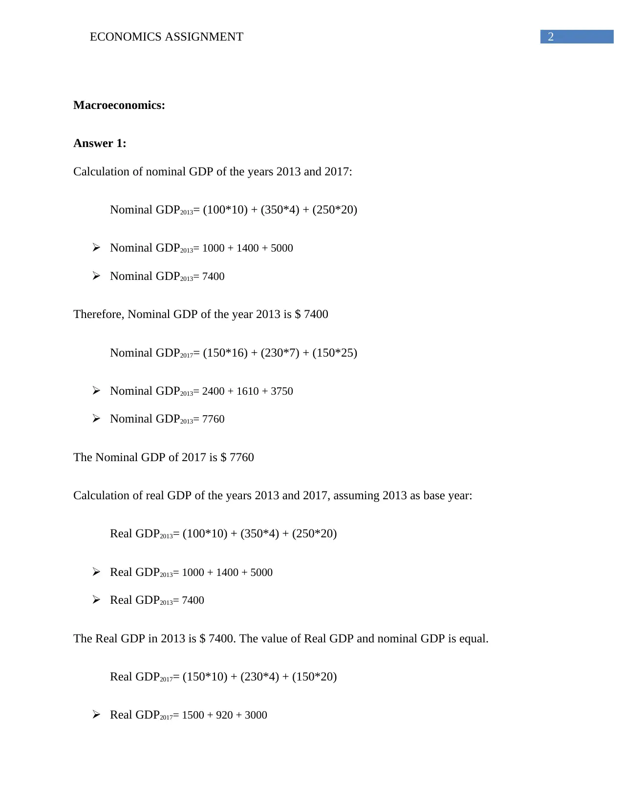
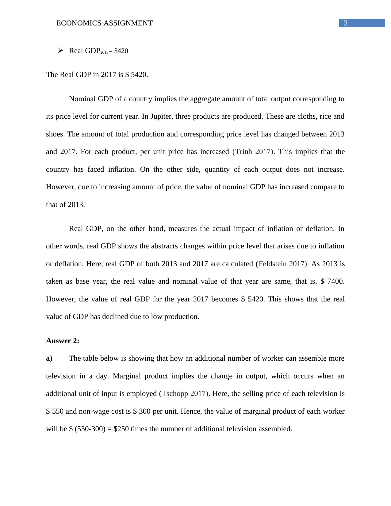
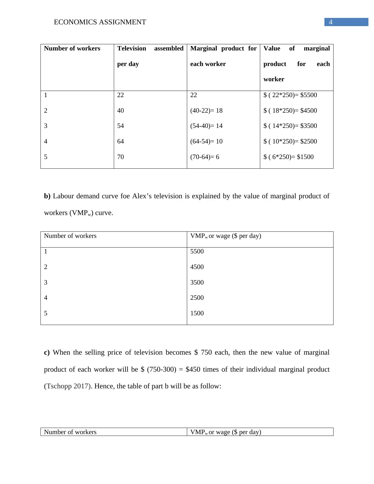
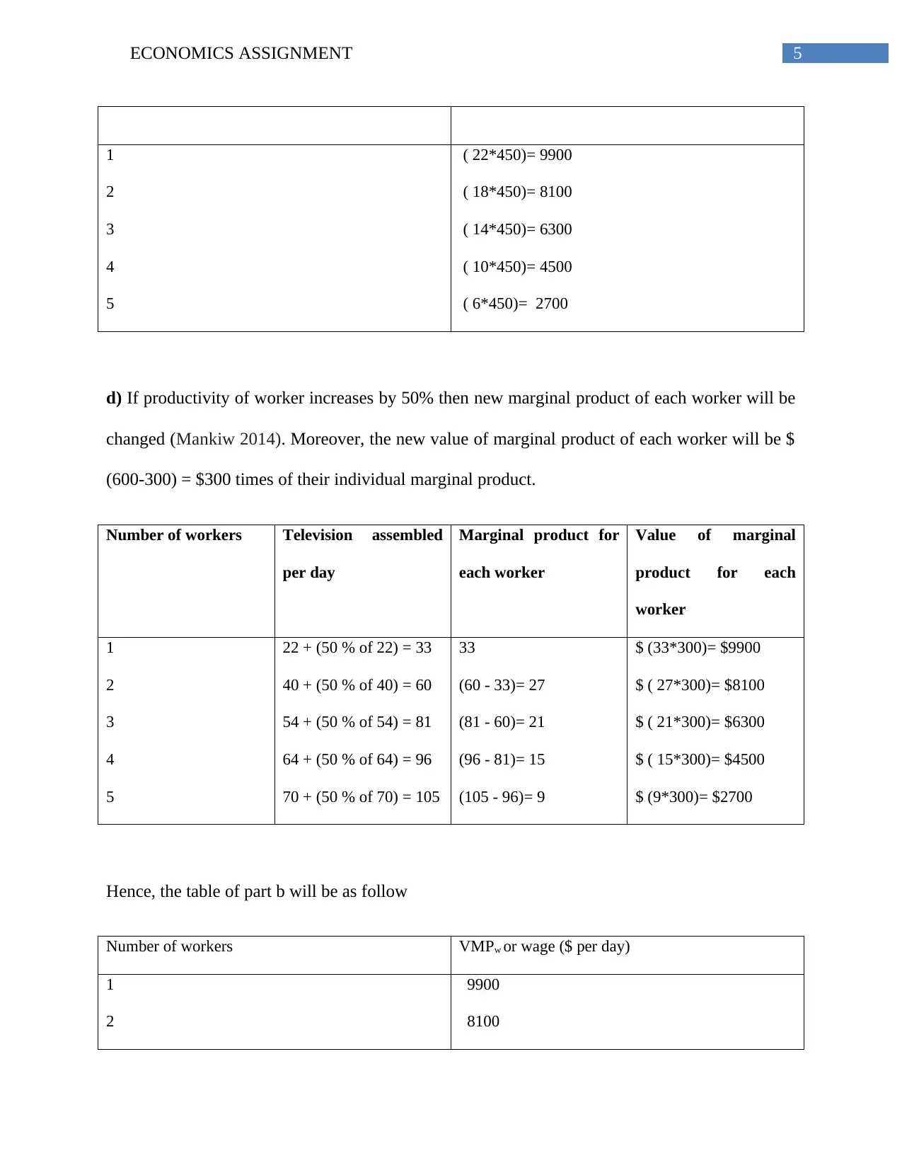
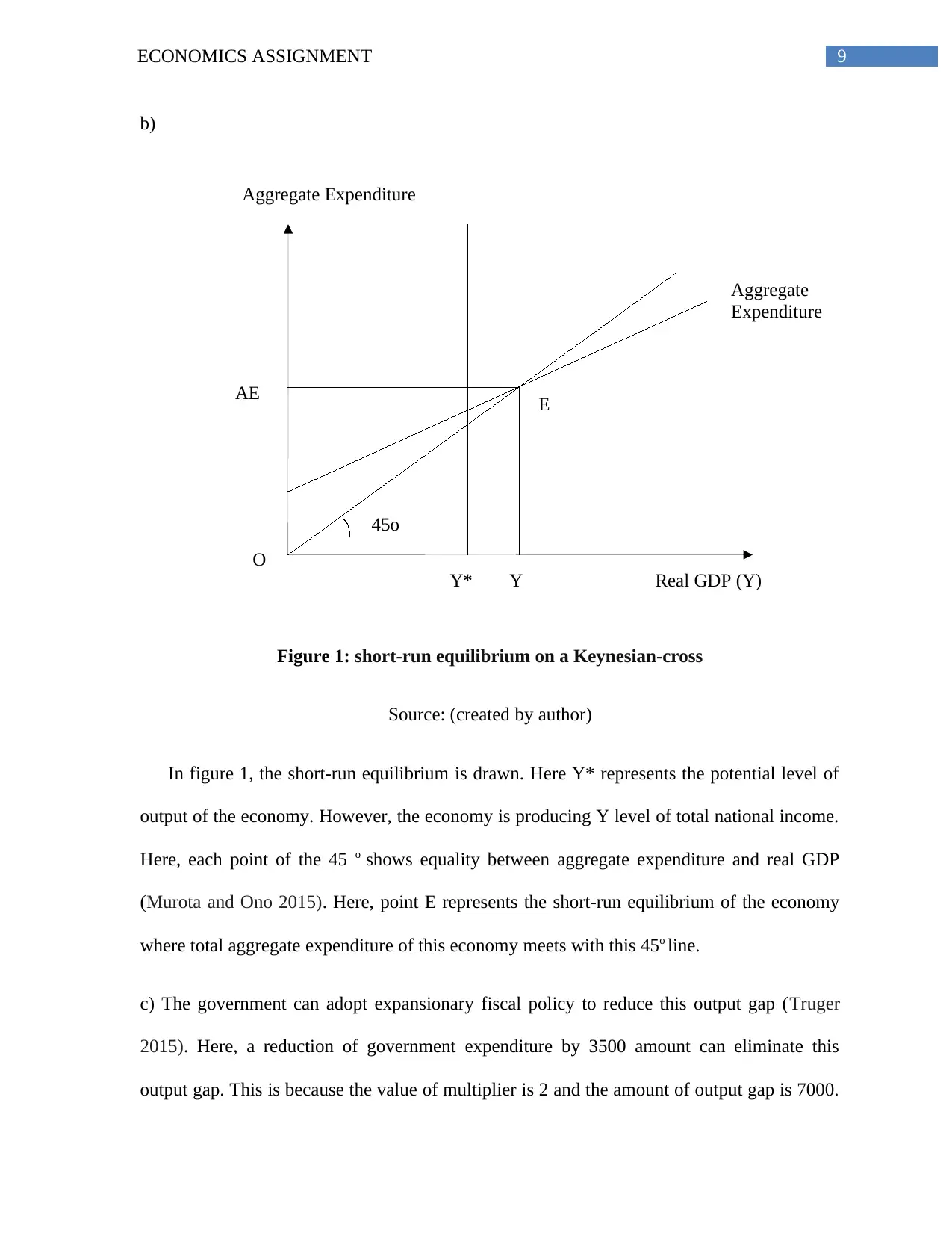
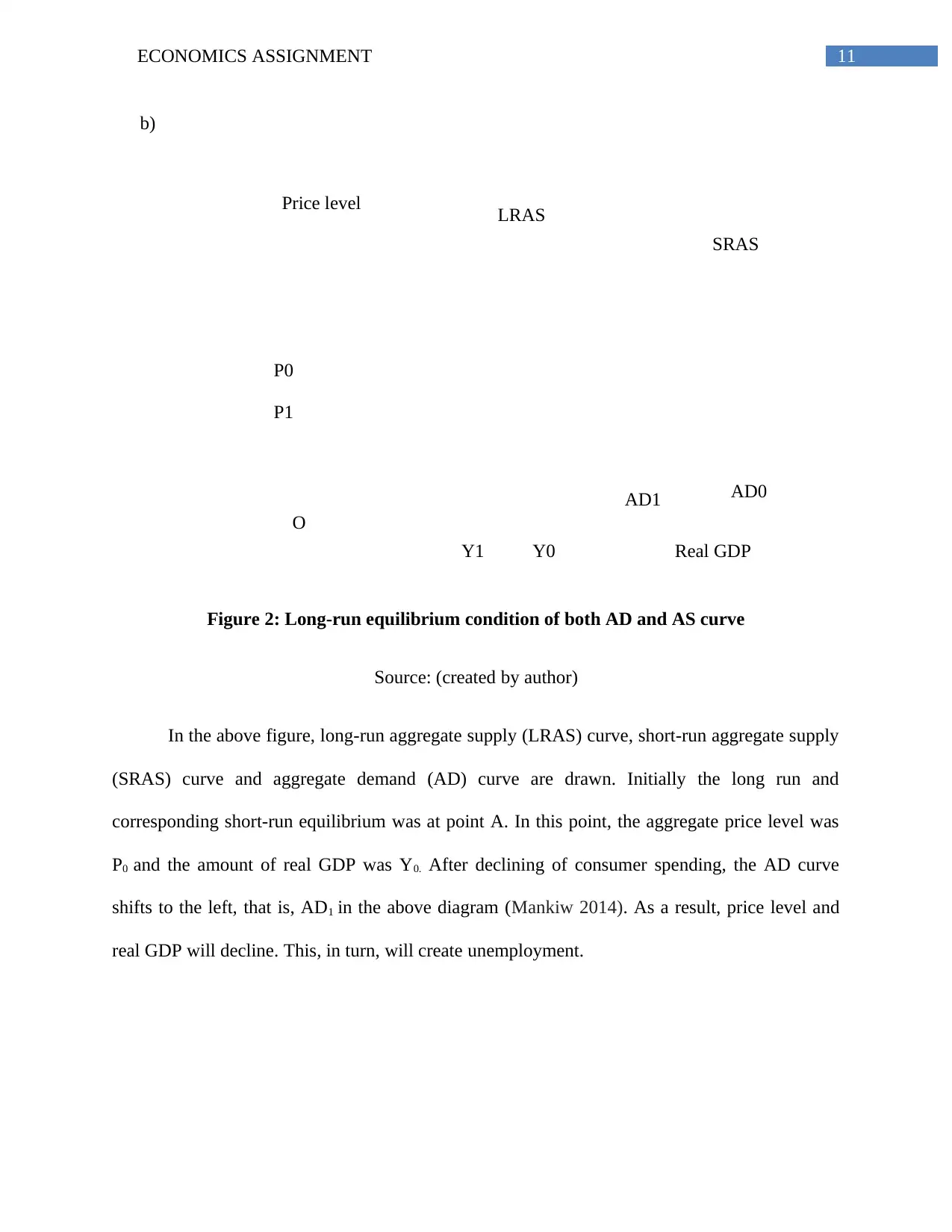
This economics assignment provides detailed solutions to questions covering both macroeconomics and microeconomics. The macroeconomics section includes calculations of nominal and real GDP for the years 2013 and 2017, analysis of labor demand curves under varying conditions (selling price of television and worker productivity), and an evaluation of John and Alice's decision to buy or rent a house based on ownership and rental costs. It also explores the calculation of autonomous expenditure, the multiplier effect, and the output gap, along with a discussion of expansionary fiscal policy. Furthermore, it discusses the impact of decreased house prices and adverse inflation shocks on aggregate demand and the role of government stabilization policies. The microeconomics section includes questions related to profit maximization strategy and the impact of supply and demand on the laptop market. Desklib provides students with access to this assignment solution and many other resources to aid in their studies.

Running head: ECONOMICS ASSIGNMENT
ECONOMICS ASSIGNMENT
Name of the university
Name of the student
Author Note

1ECONOMICS ASSIGNMENT
Table of Contents
Macroeconomics:.............................................................................................................................2
Answer 1:.....................................................................................................................................2
Answer 2:.....................................................................................................................................3
Answer 3:.....................................................................................................................................6
Answer 4:.....................................................................................................................................7
Answer 5:...................................................................................................................................10
Microeconomics:...........................................................................................................................13
Answer 1:...................................................................................................................................13
Answer 2:...................................................................................................................................13
Answer 3:...................................................................................................................................16
Answer 4:...................................................................................................................................21
Answer 5:...................................................................................................................................23
References:....................................................................................................................................24

2ECONOMICS ASSIGNMENT
Macroeconomics:
Answer 1:
Calculation of nominal GDP of the years 2013 and 2017:
Nominal GDP2013= (100*10) + (350*4) + (250*20)
 Nominal GDP2013= 1000 + 1400 + 5000
 Nominal GDP2013= 7400
Therefore, Nominal GDP of the year 2013 is $ 7400
Nominal GDP2017= (150*16) + (230*7) + (150*25)
 Nominal GDP2013= 2400 + 1610 + 3750
 Nominal GDP2013= 7760
The Nominal GDP of 2017 is $ 7760
Calculation of real GDP of the years 2013 and 2017, assuming 2013 as base year:
Real GDP2013= (100*10) + (350*4) + (250*20)
 Real GDP2013= 1000 + 1400 + 5000
 Real GDP2013= 7400
The Real GDP in 2013 is $ 7400. The value of Real GDP and nominal GDP is equal.
Real GDP2017= (150*10) + (230*4) + (150*20)
 Real GDP2017= 1500 + 920 + 3000

3ECONOMICS ASSIGNMENT
 Real GDP2013= 5420
The Real GDP in 2017 is $ 5420.
Nominal GDP of a country implies the aggregate amount of total output corresponding to
its price level for current year. In Jupiter, three products are produced. These are cloths, rice and
shoes. The amount of total production and corresponding price level has changed between 2013
and 2017. For each product, per unit price has increased (Trinh 2017). This implies that the
country has faced inflation. On the other side, quantity of each output does not increase.
However, due to increasing amount of price, the value of nominal GDP has increased compare to
that of 2013.
Real GDP, on the other hand, measures the actual impact of inflation or deflation. In
other words, real GDP shows the abstracts changes within price level that arises due to inflation
or deflation. Here, real GDP of both 2013 and 2017 are calculated (Feldstein 2017). As 2013 is
taken as base year, the real value and nominal value of that year are same, that is, $ 7400.
However, the value of real GDP for the year 2017 becomes $ 5420. This shows that the real
value of GDP has declined due to low production.
Answer 2:
a) The table below is showing that how an additional number of worker can assemble more
television in a day. Marginal product implies the change in output, which occurs when an
additional unit of input is employed (Tschopp 2017). Here, the selling price of each television is
$ 550 and non-wage cost is $ 300 per unit. Hence, the value of marginal product of each worker
will be $ (550-300) = $250 times the number of additional television assembled.

4ECONOMICS ASSIGNMENT
Number of workers Television assembled
per day
Marginal product for
each worker
Value of marginal
product for each
worker
1
2
3
4
5
22
40
54
64
70
22
(40-22)= 18
(54-40)= 14
(64-54)= 10
(70-64)= 6
$ ( 22*250)= $5500
$ ( 18*250)= $4500
$ ( 14*250)= $3500
$ ( 10*250)= $2500
$ ( 6*250)= $1500
b) Labour demand curve foe Alex’s television is explained by the value of marginal product of
workers (VMPw) curve.
Number of workers VMPw or wage ($ per day)
1
2
3
4
5
5500
4500
3500
2500
1500
c) When the selling price of television becomes $ 750 each, then the new value of marginal
product of each worker will be $ (750-300) = $450 times of their individual marginal product
(Tschopp 2017). Hence, the table of part b will be as follow:
Number of workers VMPw or wage ($ per day)

5ECONOMICS ASSIGNMENT
1
2
3
4
5
( 22*450)= 9900
( 18*450)= 8100
( 14*450)= 6300
( 10*450)= 4500
( 6*450)= 2700
d) If productivity of worker increases by 50% then new marginal product of each worker will be
changed (Mankiw 2014). Moreover, the new value of marginal product of each worker will be $
(600-300) = $300 times of their individual marginal product.
Number of workers Television assembled
per day
Marginal product for
each worker
Value of marginal
product for each
worker
1
2
3
4
5
22 + (50 % of 22) = 33
40 + (50 % of 40) = 60
54 + (50 % of 54) = 81
64 + (50 % of 64) = 96
70 + (50 % of 70) = 105
33
(60 - 33)= 27
(81 - 60)= 21
(96 - 81)= 15
(105 - 96)= 9
$ (33*300)= $9900
$ ( 27*300)= $8100
$ ( 21*300)= $6300
$ ( 15*300)= $4500
$ (9*300)= $2700
Hence, the table of part b will be as follow
Number of workers VMPw or wage ($ per day)
1
2
9900
8100

6ECONOMICS ASSIGNMENT
3
4
5
6300
4500
2700
Answer 3:
a) John and Alice’s ownership costs equal their general expenses (maintenances, taxes and
insurance) and their mortgage interest costs (Sommer and Sullivan 2018). General expenses are
4% of $250,000 = $ 10,000 per year and interest expenses are 6% of $250,000= $ 15,000 per
year. Therefore, the total ownership cost is $ (10,000 + 15,000) = $25,000 per year. This exceeds
the cost of renting, that is, $1800 per month for 12 months or $(1,800*12) = $ 21,600. Therefore,
John and Alice should rent rather than buy.
b) If they are willing to pay $ 2,500 as monthly rent then their rental cost will be $(2,500*12) =
$30,000 per year. In this situation, the rental charge is exceeding the ownership cost. Hence, they
should buy a new house.
c) If the rental interest becomes 4% then interest expenses will be 4% of $ 250,000 = $10,000.
Hence, the ownership cost will be $ (10,000+ 10,000) = $ 20,000. This ownership cost is lower
compare to the cost of renting, that is, $ 21,600. Hence, they should buy the house.
d) General expenses are 4% of $200,000 = $ 8,000 per year and interest expenses are 6% of
$200,000= $ 12,000 per year. Therefore, the total ownership cost is $ (8,000 + 12,000) = $20,000
per year. This amount is lower compare the cost of renting cost $ 21,600. Therefore, John and
Alice should buy the new house.

7ECONOMICS ASSIGNMENT
e) Due to high rate of interest, the ownership cost becomes high. As a result, buyers cannot buy
house. If this rate of interest remains low then the ownership cost will also be low. It will further
increase the demand of house (Favilukis, Ludvigson and Van Nieuwerburgh 2017). Home-
building companies always try to sell houses to their affordable customers. However, high rate of
interest influenced their business negatively. Thus, home-building companies dislike high rate of
interests.
Answer 4:
a) To calculate autonomous expenditure of an economy, some specific components of national
income or national expenditure will be considered (Mankiw 2014). Thos autonomous parts are
not influenced by the national income of that economy.
Here, the given equation of consumption is C = 6,000 + 0.5 (Y-T). The autonomous part
of consumption is 6,000. Investment (I) = 2000, Government expenditure (G) = 4500, net export
(NX) = 500 and tax (T) = 4000.
Hence, autonomous expenditure = C + I + G + NX + T
 autonomous expenditure = 6000 + 2000 + 4500 + 500 + 4000
 autonomous expenditure = 17000
The value of multiplier will be 1/ (1 – MPC), where MPC indicates marginal propensity
to consume. Hence, the multiplier will be 1/ (1- 0.5) = 1/ 0.5 = 2
Short-run equilibrium output will be Y= C + I +G +T +NX
Y= 6,000 + 0.5 (Y-T) + 2000 + 4500 + 4000 + 500
 Y= 0.5 Y – 0.5 T + 17000

8ECONOMICS ASSIGNMENT
 Y = 0.5 Y – 0.5 * 4000 + 17000
 Y = 0.5 Y + 15000
 (1 – 0.5) Y = 15000
 0.5 Y = 15000
 Y= 15000/0.5
 Y = 30000
The potential output of this economy is Y* = 23,000
Hence, the output gap is:
(Y-Y*) = 30,000-23000
 (Y- Y*) = 7,000
Therefore, the economy is facing an expansionary gap of output by 7,000.

9ECONOMICS ASSIGNMENT
Y* Y
45o
Real GDP (Y)
Aggregate
Expenditure
Aggregate Expenditure
O
E
AE
b)
Figure 1: short-run equilibrium on a Keynesian-cross
Source: (created by author)
In figure 1, the short-run equilibrium is drawn. Here Y* represents the potential level of
output of the economy. However, the economy is producing Y level of total national income.
Here, each point of the 45 o shows equality between aggregate expenditure and real GDP
(Murota and Ono 2015). Here, point E represents the short-run equilibrium of the economy
where total aggregate expenditure of this economy meets with this 45o line.
c) The government can adopt expansionary fiscal policy to reduce this output gap (Truger
2015). Here, a reduction of government expenditure by 3500 amount can eliminate this
output gap. This is because the value of multiplier is 2 and the amount of output gap is 7000.

10ECONOMICS ASSIGNMENT
Multiplier analysis will help to determine the relationship between government expenditure
and real GDP. Hence, using those values in government expenditure multiplier, the amount
of reduction will be obtained.
d) In case of tax, a change in tax does not imply the change of autonomous part of tax. It will
only change cdT amount where, c is MPC. Here, tax multiplier analysis will again help to
determine the relation between tax and real GDP (Mankiw 2014). Tax multiplier: dY/dT = -
(1-m)/ m, where, m is MPC. The government will increase tax by $10.
Answer 5:
a) In the long-run equilibrium, due to decrease in house prices, consumers also decrease
their spending (Mankiw 2014). This will shift the aggregate demand curve (AD) to the left.

11ECONOMICS ASSIGNMENT
Price level
Real GDP
O
LRAS
SRAS
AD0AD1
P0
P1
Y0Y1
b)
Figure 2: Long-run equilibrium condition of both AD and AS curve
Source: (created by author)
In the above figure, long-run aggregate supply (LRAS) curve, short-run aggregate supply
(SRAS) curve and aggregate demand (AD) curve are drawn. Initially the long run and
corresponding short-run equilibrium was at point A. In this point, the aggregate price level was
P0 and the amount of real GDP was Y0. After declining of consumer spending, the AD curve
shifts to the left, that is, AD1 in the above diagram (Mankiw 2014). As a result, price level and
real GDP will decline. This, in turn, will create unemployment.