Economics Study Material

This document provides study material for economics, including solved assignments and essays. It covers topics such as production possibilities frontier, demand and supply curves, price elasticity of demand, and more. The content is relevant for economics courses at various universities.

Running head: ECONOMICS
Economics
Name of the Student
Name of the University
Course ID

1ECONOMICS
Table of Contents
Question 1..................................................................................................................................2
Question a...............................................................................................................................2
Question b..............................................................................................................................2
Question c...............................................................................................................................3
Question d..............................................................................................................................3
Question 2..................................................................................................................................4
Question a...............................................................................................................................4
Question b..............................................................................................................................4
Question c...............................................................................................................................5
Question e...............................................................................................................................6
Question 3..................................................................................................................................7
Question a...............................................................................................................................7
Question b..............................................................................................................................8
Question c...............................................................................................................................8
Question d..............................................................................................................................8
Question e...............................................................................................................................8
Question f...............................................................................................................................8
Question g..............................................................................................................................9
Question h............................................................................................................................10
Question 4................................................................................................................................10
Question a.............................................................................................................................10
Question b............................................................................................................................11
Question c.............................................................................................................................11
Question d............................................................................................................................12
Question 5................................................................................................................................12
Question a.............................................................................................................................12
Question b............................................................................................................................13
Question c.............................................................................................................................13
Question d............................................................................................................................13
Question e.............................................................................................................................13
References................................................................................................................................14

2ECONOMICS
Question 1
Question a
0 100 200 300 400 500 600 700 800 900 1000 1100 1200 1300 1400 1500 1600 1700 1800 1900
0
170
340
510
680
850
1020
1190
1360
Production Possibilities Frontier (PPF)
Semillon
Semillon Chardonnay
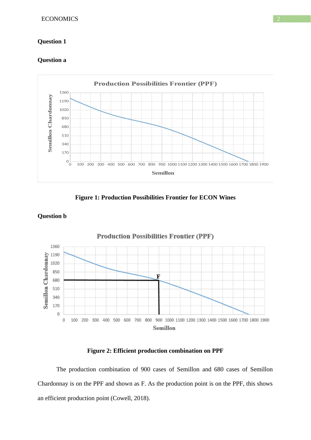
Figure 1: Production Possibilities Frontier for ECON Wines
Question b
Figure 2: Efficient production combination on PPF
The production combination of 900 cases of Semillon and 680 cases of Semillon
Chardonnay is on the PPF and shown as F. As the production point is on the PPF, this shows
an efficient production point (Cowell, 2018).

3ECONOMICS
Question c
Natural calamities like drought destroys economic resources. The destruction of
resources hamper production of all the goods in the economy. The lower availability of
resources to all industry reduces output and shifts the PPF inward.
Question d
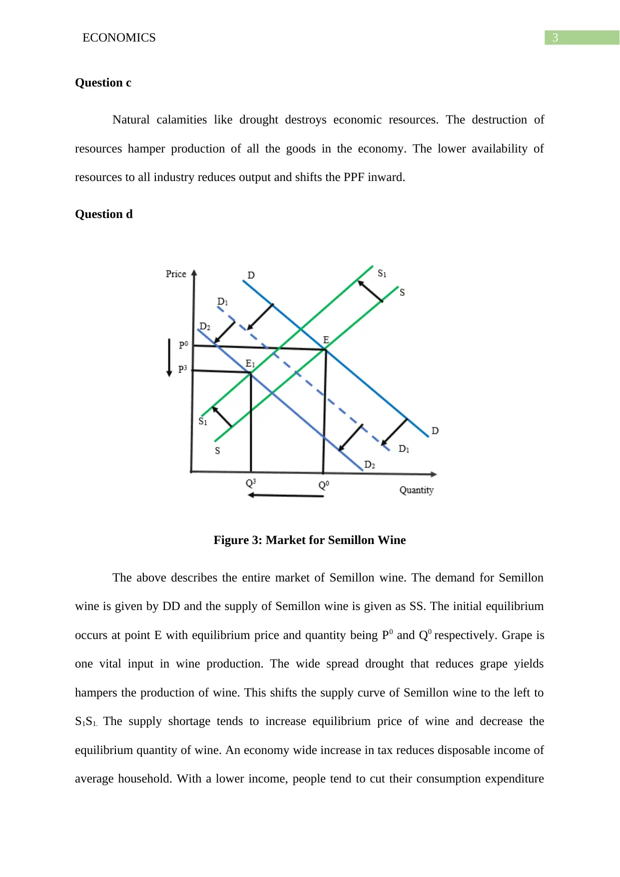
Figure 3: Market for Semillon Wine
The above describes the entire market of Semillon wine. The demand for Semillon
wine is given by DD and the supply of Semillon wine is given as SS. The initial equilibrium
occurs at point E with equilibrium price and quantity being P0 and Q0 respectively. Grape is
one vital input in wine production. The wide spread drought that reduces grape yields
hampers the production of wine. This shifts the supply curve of Semillon wine to the left to
S1S1. The supply shortage tends to increase equilibrium price of wine and decrease the
equilibrium quantity of wine. An economy wide increase in tax reduces disposable income of
average household. With a lower income, people tend to cut their consumption expenditure

4ECONOMICS
(Friedman, 2017). As a result, the demand of wine will be reduced as shown by the inward of
supply curve from DD to D1D1. Demand of wine further reduces following a decrease in price
of beer. As beer and wine are substitute a decrease in price of beer encourages people to
consume more beer while discouraging consumption of wine. The demand curve of wine
again shifts leftward to D2D2. The lower demand causes a downward pressure on price. The
final equilibrium occurs where the new supply curve and new demand curve intersects. The
effect on equilibrium price depends on magnitude of change in demand and supply. As
change in demand far exceeds the change in supply, equilibrium price lowers to P3 and
equilibrium quantity lowers to Q3.
Question 2
Question a
Price
Quantit
y of
tickets
sold per
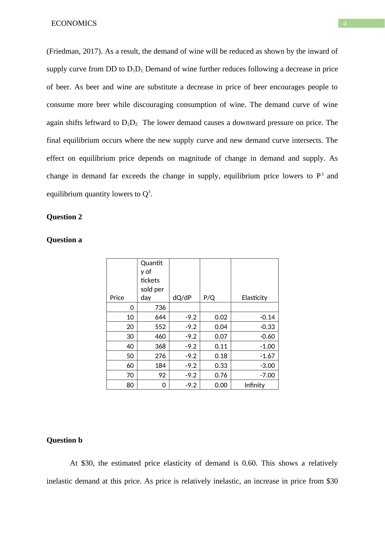
day dQ/dP P/Q Elasticity
0 736
10 644 -9.2 0.02 -0.14
20 552 -9.2 0.04 -0.33
30 460 -9.2 0.07 -0.60
40 368 -9.2 0.11 -1.00
50 276 -9.2 0.18 -1.67
60 184 -9.2 0.33 -3.00
70 92 -9.2 0.76 -7.00
80 0 -9.2 0.00 Infinity
Question b
At $30, the estimated price elasticity of demand is 0.60. This shows a relatively
inelastic demand at this price. As price is relatively inelastic, an increase in price from $30

5ECONOMICS
will increase revenue of the theatre company. Because of inelastic nature of demand, the
proportionate decrease in demand following the increase in price is less than the
proportionate increase in price (Baumol & Blinder, 2015). This results in an increase in
revenue following a price increase.
Question c
The obtained equation for daily demand for theatre ticket is
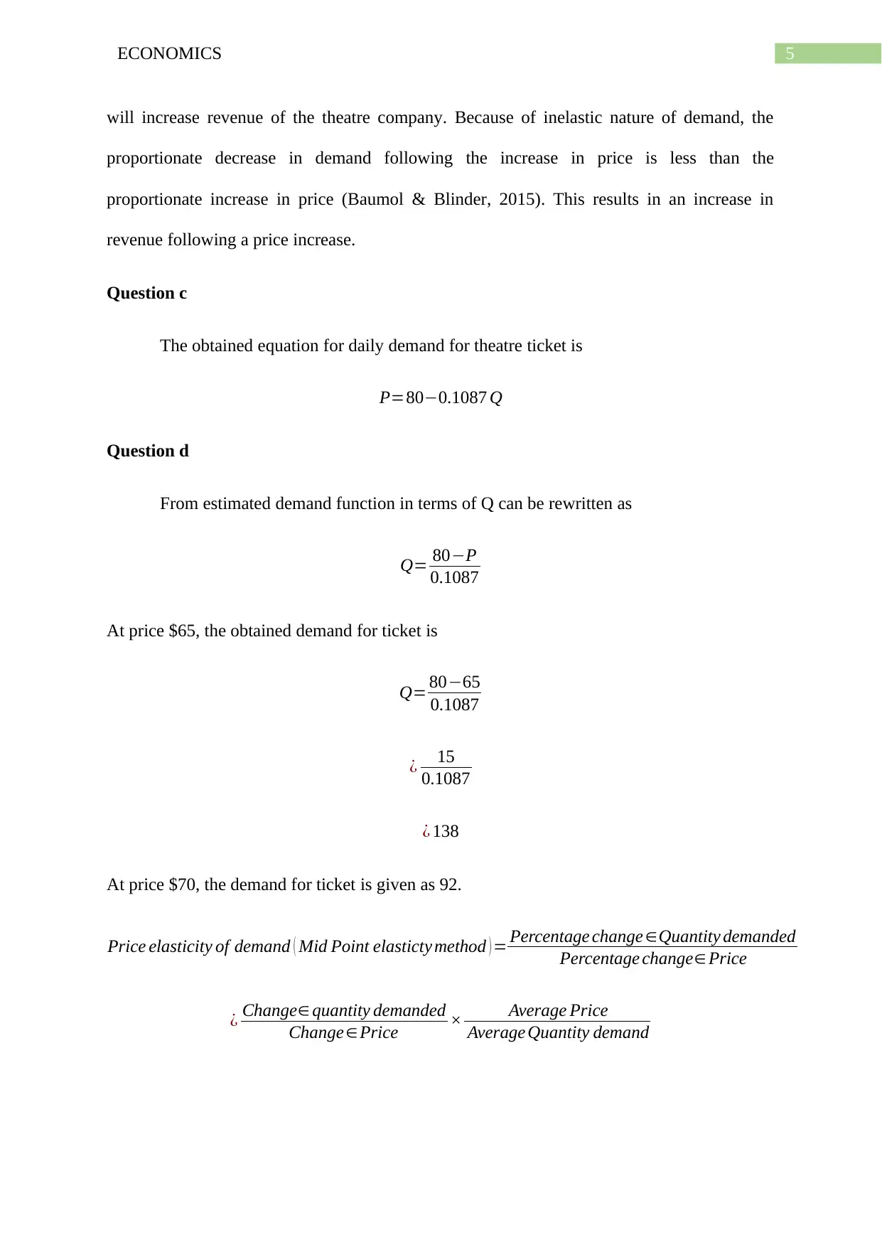
P=80−0.1087 Q
Question d
From estimated demand function in terms of Q can be rewritten as
Q= 80−P
0.1087
At price $65, the obtained demand for ticket is
Q= 80−65
0.1087
¿ 15
0.1087
¿ 138
At price $70, the demand for ticket is given as 92.
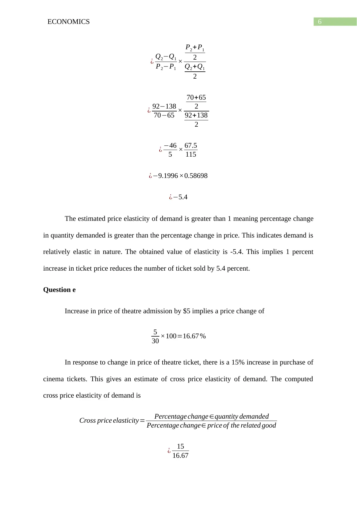
Price elasticity of demand ( Mid Point elasticty method ) = Percentage change ∈Quantity demanded
Percentage change∈ Price
¿ Change∈ quantity demanded
Change∈Price × Average Price
Average Quantity demand

6ECONOMICS
¿ Q2−Q1
P2−P1
×
P2 + P1
2
Q2 +Q1
2
¿ 92−138
70−65 ×
70+65
2
92+138
2
¿ −46
5 × 67.5
115
¿−9.1996 ×0.58698
¿−5.4
The estimated price elasticity of demand is greater than 1 meaning percentage change
in quantity demanded is greater than the percentage change in price. This indicates demand is
relatively elastic in nature. The obtained value of elasticity is -5.4. This implies 1 percent
increase in ticket price reduces the number of ticket sold by 5.4 percent.
Question e
Increase in price of theatre admission by $5 implies a price change of
5
30 ×100=16.67 %
In response to change in price of theatre ticket, there is a 15% increase in purchase of
cinema tickets. This gives an estimate of cross price elasticity of demand. The computed
cross price elasticity of demand is
Cross price elasticity= Percentage change ∈quantity demanded
Percentage change∈ price of the related good
¿ 15
16.67

7ECONOMICS
¿ 0. 90
The obtained cross price elasticity shows that 1 percent increase in price of cinema
theatre admission increases demand for cinema tickets by 0.9 percent.
The elasticity value tells the cinema managers that theatre ticket price and cinema
tickets are substitutes (Cowen & Tabarrok, 2015).
Given the information that increase in price results in a 15% increase in purchase of
cinema tickets, number of cinema tickets purchased after increase in ticket price of theatre is
obtained as
350+ ( 350 ×15 % )
¿ 350+52.5
¿ 402.5 403
Question 3
Question a
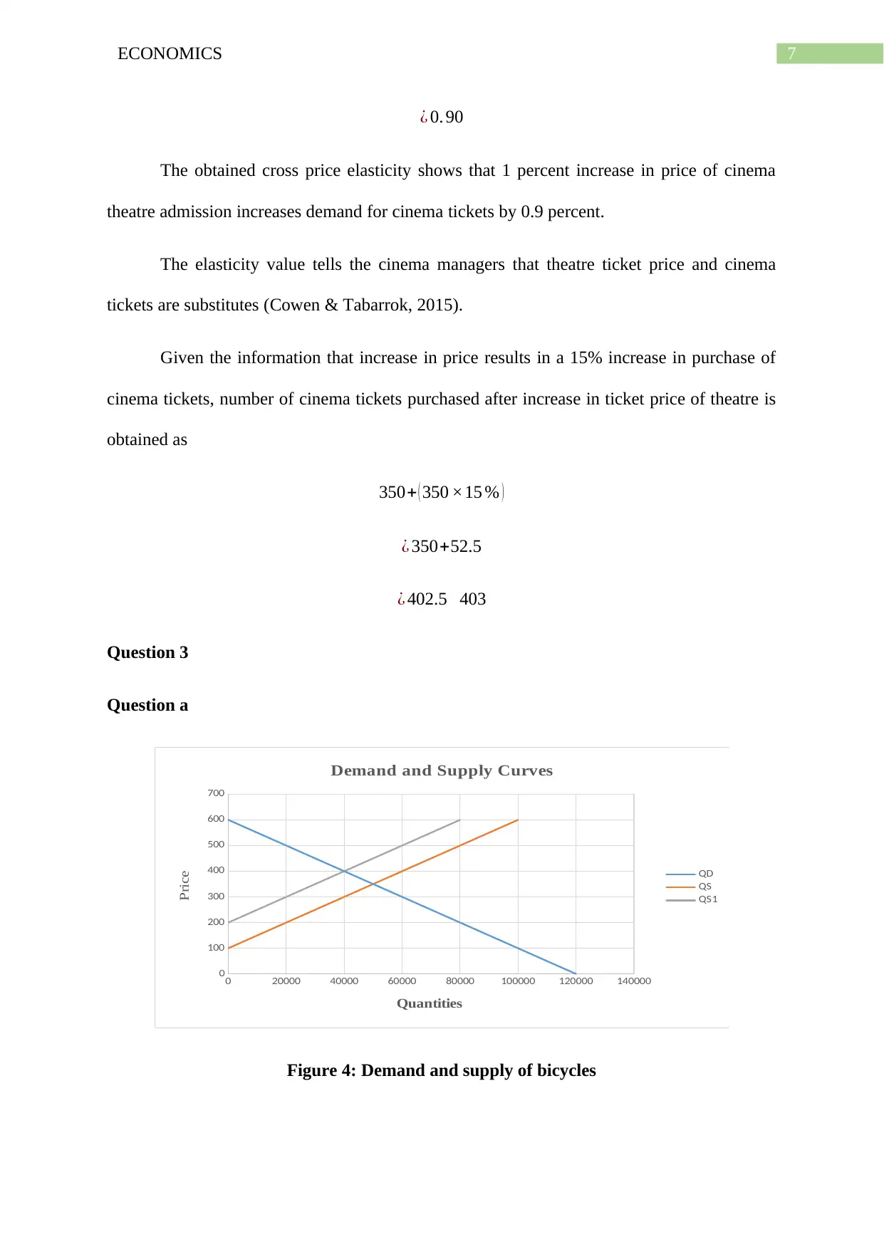
0 20000 40000 60000 80000 100000 120000 140000
0
100
200
300
400
500
600
700
Demand and Supply Curves
QD
QS
QS1
Quantities
Price
Figure 4: Demand and supply of bicycles

8ECONOMICS
Question b
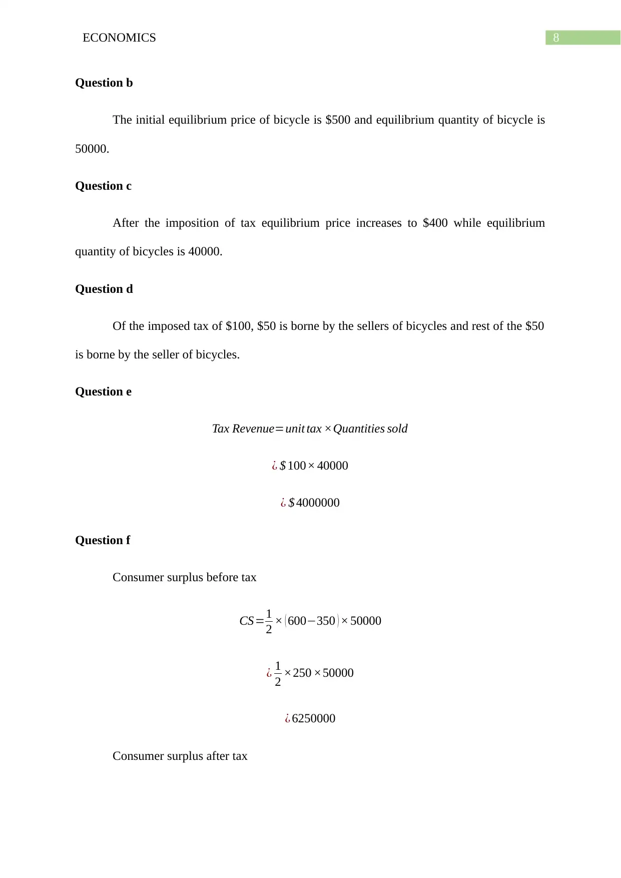
The initial equilibrium price of bicycle is $500 and equilibrium quantity of bicycle is
50000.
Question c
After the imposition of tax equilibrium price increases to $400 while equilibrium
quantity of bicycles is 40000.
Question d
Of the imposed tax of $100, $50 is borne by the sellers of bicycles and rest of the $50
is borne by the seller of bicycles.
Question e
Tax Revenue=unit tax ×Quantities sold
¿ $ 100× 40000
¿ $ 4000000
Question f
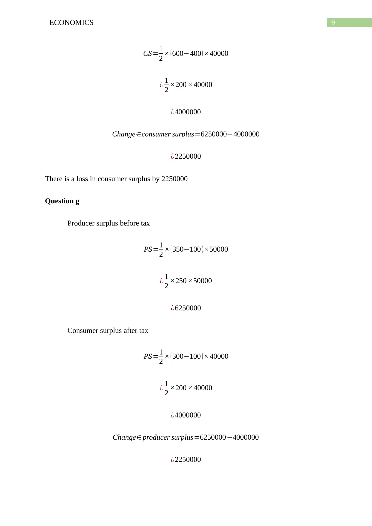
Consumer surplus before tax
CS=1
2 × ( 600−350 ) × 50000
¿ 1
2 ×250 ×50000
¿ 6250000
Consumer surplus after tax

9ECONOMICS
CS=1
2 × ( 600−400 ) ×40000
¿ 1
2 ×200 × 40000
¿ 4000000
Change∈consumer surplus=6250000−4000000
¿ 2250000
There is a loss in consumer surplus by 2250000
Question g
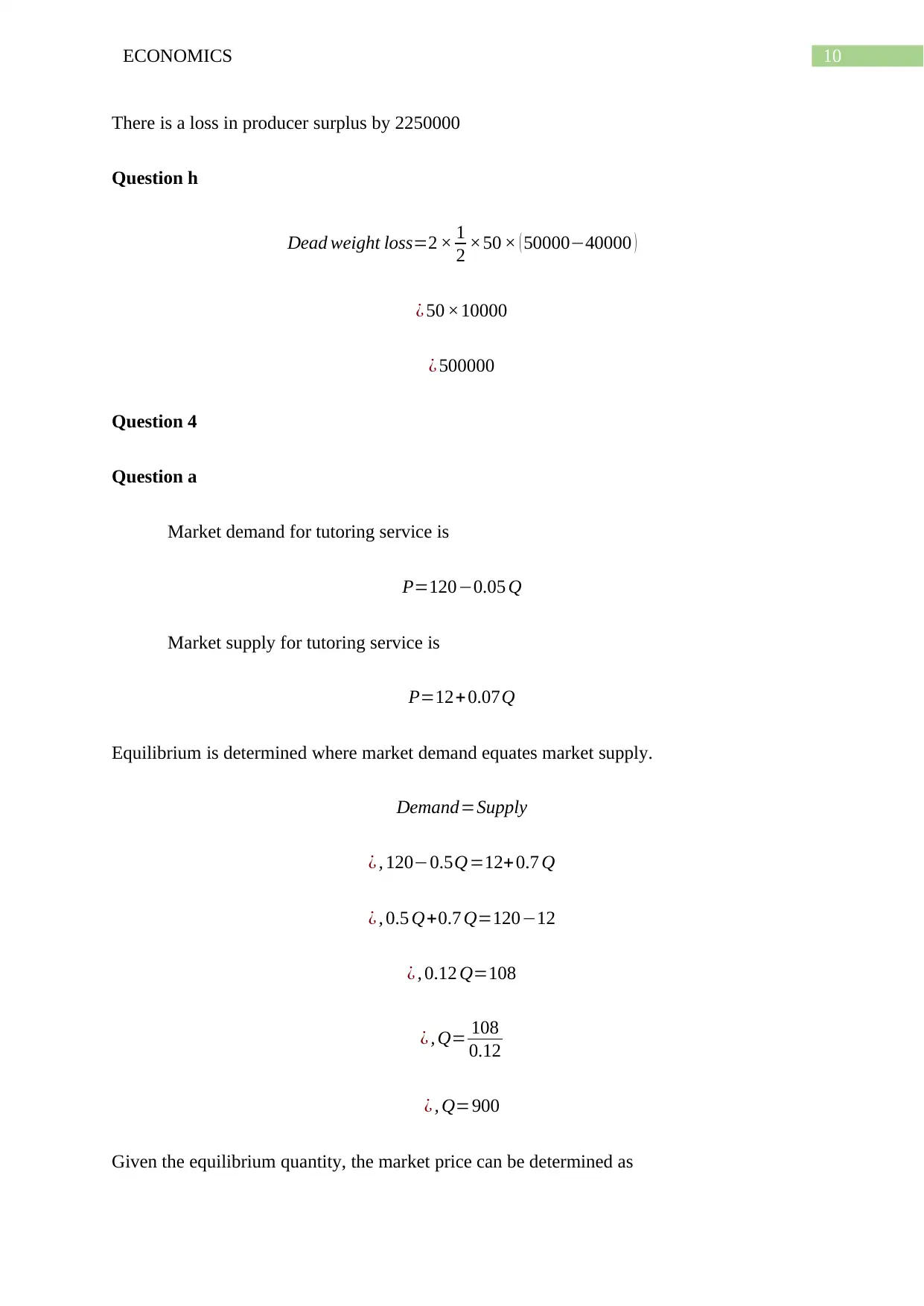
Producer surplus before tax
PS=1
2 × ( 350−100 ) ×50000
¿ 1
2 ×250 ×50000
¿ 6250000
Consumer surplus after tax
PS=1
2 × ( 300−100 ) × 40000
¿ 1
2 ×200 × 40000
¿ 4000000
Change∈ producer surplus=6250000−4000000
¿ 2250000

10ECONOMICS
There is a loss in producer surplus by 2250000
Question h
Dead weight loss=2 × 1
2 ×50 × ( 50000−40000 )
¿ 50 ×10000
¿ 500000
Question 4
Question a
Market demand for tutoring service is
P=120−0.05 Q
Market supply for tutoring service is
P=12+0.07Q
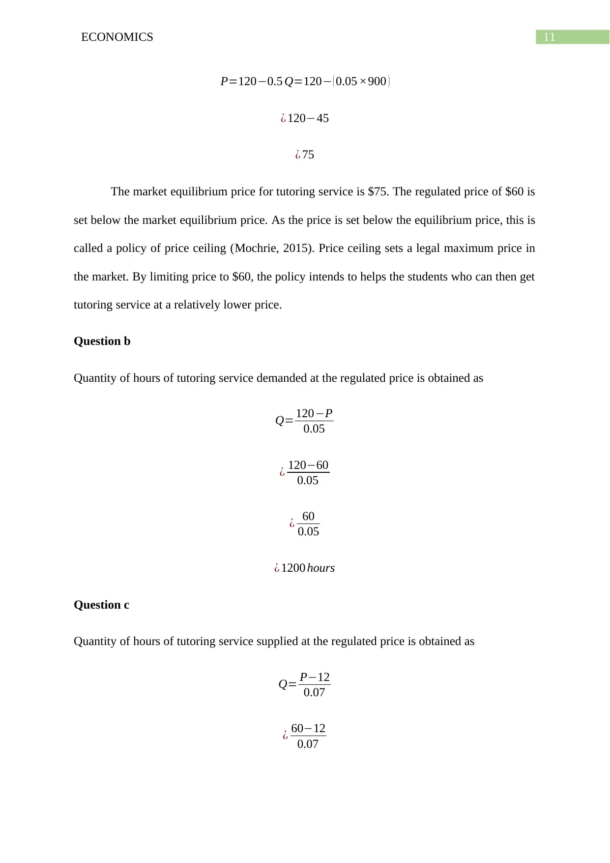
Equilibrium is determined where market demand equates market supply.
Demand=Supply
¿ , 120−0.5Q=12+0.7 Q
¿ , 0.5 Q+0.7 Q=120−12
¿ , 0.12 Q=108
¿ , Q= 108
0.12
¿ , Q=900
Given the equilibrium quantity, the market price can be determined as

11ECONOMICS
P=120−0.5 Q=120− ( 0.05 ×900 )
¿ 120−45
¿ 75
The market equilibrium price for tutoring service is $75. The regulated price of $60 is
set below the market equilibrium price. As the price is set below the equilibrium price, this is
called a policy of price ceiling (Mochrie, 2015). Price ceiling sets a legal maximum price in
the market. By limiting price to $60, the policy intends to helps the students who can then get
tutoring service at a relatively lower price.
Question b
Quantity of hours of tutoring service demanded at the regulated price is obtained as
Q= 120−P
0.05
¿ 120−60
0.05
¿ 60
0.05
¿ 1200 hours
Question c
Quantity of hours of tutoring service supplied at the regulated price is obtained as
Q= P−12
0.07
¿ 60−12
0.07

12ECONOMICS
¿ 48
0.07
¿ 685.71 686 hours
Question d
Figure 5: Economic surplus resulted from regulated price
Question 5
Question a
Numbe
r of
worker
s
Output(unit
s)
Margin
al
Product
of
Labour
Fixed
cost
(Capital
)
Varible
Cost
(labour
)
Total
Cost
Margin
al Cost
Averag
e Fixed
Costs
Averag
e
Variabl
e Costs
Averag
e Total
Costs
0 0 - $600 0 $600 - - - -
1 330 330 $600 $300 $900 $300 $600 $300 $900
2 705 375 $600 $600
$1,20
0 $300 $300 $300 $600
3 1020 315 $600 $900
$1,50
0 $300 $200 $300 $500
4 1260 240 $600 $1,200 $1,80 $300 $150 $300 $450

13ECONOMICS
0
5 1410 150 $600 $1,500
$2,10
0 $300 $120 $300 $420
6 1470 60 $600 $1,800
$2,40
0 $300 $100 $300 $400
Question b
Firm’s revenue corresponding to break even is $900. At break-even total revenue
equals total cost. Total cost of the firm is $900 corresponding to the output level of 330.
Question c
The diminishing return occurs from the output level of 1020 units. From this level of
output, the marginal product of labor starts falling indicating adding one additional labor
would make a relatively smaller addition to total output (Mankiw, 2016). This is because
given the fixed supply of capital, addition more and more labor reduces capital per worker
and hence, reduces marginal product of labor.
Question d
Following the trend in marginal product of labor, the marginal product of labor is
negative corresponding to the output level of 2000 units. The firm should not commit to the
order unless there is room for hiring additional labor, which might results in positive return
from the additional labor unit.
Question e

14ECONOMICS
330 530 730 930 1130 1330 1530
$0
$100
$200
$300
$400
$500
$600
$700
$800
$900
$1,000
AVC, ATC, MC and AFC
Marginal Cost
Average Fixed Costs
Average Variable Costs
Average Total Costs
Figure 6: Average variable cost, average total cost, marginal cost and average fixed cost
Fixed cost refers to the cost that does not vary with level of output. This costs are
independent of level of output (Mahanty, 2014). This is the cost associated with fixed inputs.
Labor being a variable unit, an increase in labor cost will not make any change to average
fixed cost and hence, it will not shift.
Variables cost are costs that depend on the level of output. As labor is the variable
input an increase in labor cost will increase the average variable cost shifting the curve up.
With increase in average variable cost average total cost which is the sum of average
fixed cost and average variable cost will increase as well. The average total cost will shift
upward.
Marginal cost is the change in total cost due to unit change in output (Kreps, 2019).
Following an increase in cost of labor, marginal cost increases causing the existing marginal
cost curve up.

15ECONOMICS
References
Baumol, W. J., & Blinder, A. S. (2015). Microeconomics: Principles and policy. Nelson
Education.
Cowell, F. (2018). Microeconomics: principles and analysis. Oxford University Press.
Cowen, T., & Tabarrok, A. (2015). Modern principles of microeconomics. Macmillan
International Higher Education.
Friedman, L. S. (2017). The microeconomics of public policy analysis. Princeton University
Press.
Kreps, D. M. (2019). Microeconomics for managers. Princeton University Press.
Mahanty, A. K. (2014). Intermediate microeconomics with applications. Academic Press.
Mankiw, N. G. (2016). Principle of Microeconomics. Cengage Learning.
Mochrie, R. (2015). Intermediate microeconomics. Macmillan International Higher
Education.