Economics: GDP, Consumption, and Government Expenditure

This document discusses the concepts of GDP, consumption, and government expenditure in economics. It explains the calculation of actual GDP and the components of consumption function. It also explores the impact of fiscal and monetary policies on economic stability. Additionally, it analyzes the effects of the China-US trade war on Australia's economy.

Running head: ECONOMICS
Economics
Name of the Student
Name of the University
Student ID

1ECONOMICS
Table of Contents
Problem............................................................................................................................................2
Part (a).........................................................................................................................................2
Part (b).........................................................................................................................................3
Part (c).........................................................................................................................................4
Part (d).........................................................................................................................................4
Part (e).........................................................................................................................................5
Part (f)..........................................................................................................................................6
Part (g).........................................................................................................................................7
Part (h).........................................................................................................................................8
Part (i)........................................................................................................................................10
Part (j)........................................................................................................................................10
List of references...........................................................................................................................12

2ECONOMICS
Problem
Part (a)
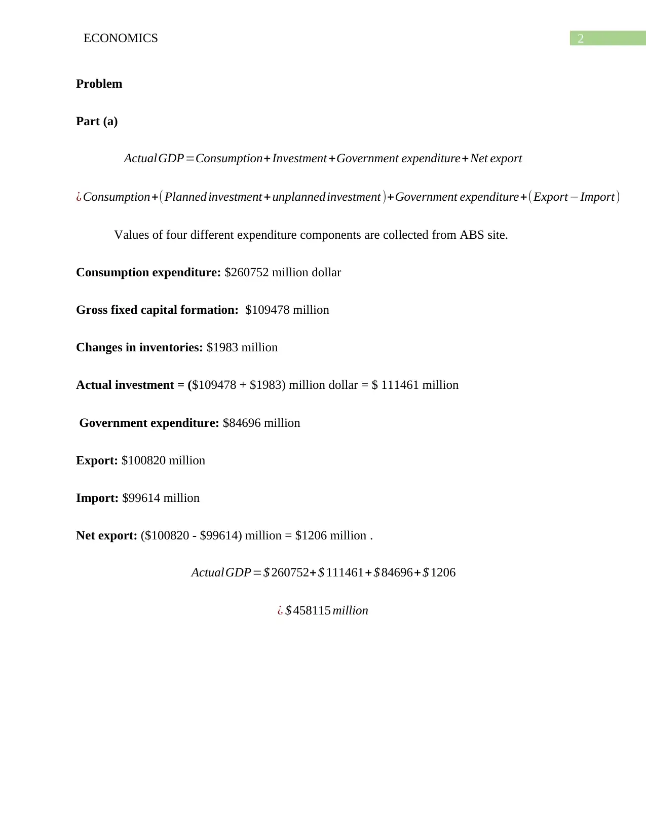
ActualGDP=Consumption+ Investment +Government expenditure+Net export
¿ Consumption+( Planned investment + unplanned investment )+Government expenditure+(Export−Import)
Values of four different expenditure components are collected from ABS site.
Consumption expenditure: $260752 million dollar
Gross fixed capital formation: $109478 million
Changes in inventories: $1983 million
Actual investment = ($109478 + $1983) million dollar = $ 111461 million
Government expenditure: $84696 million
Export: $100820 million
Import: $99614 million
Net export: ($100820 - $99614) million = $1206 million .
ActualGDP=$ 260752+ $ 111461+ $ 84696+ $ 1206
¿ $ 458115 million

3ECONOMICS
Part (b)
Standard form of a consumption function is given as
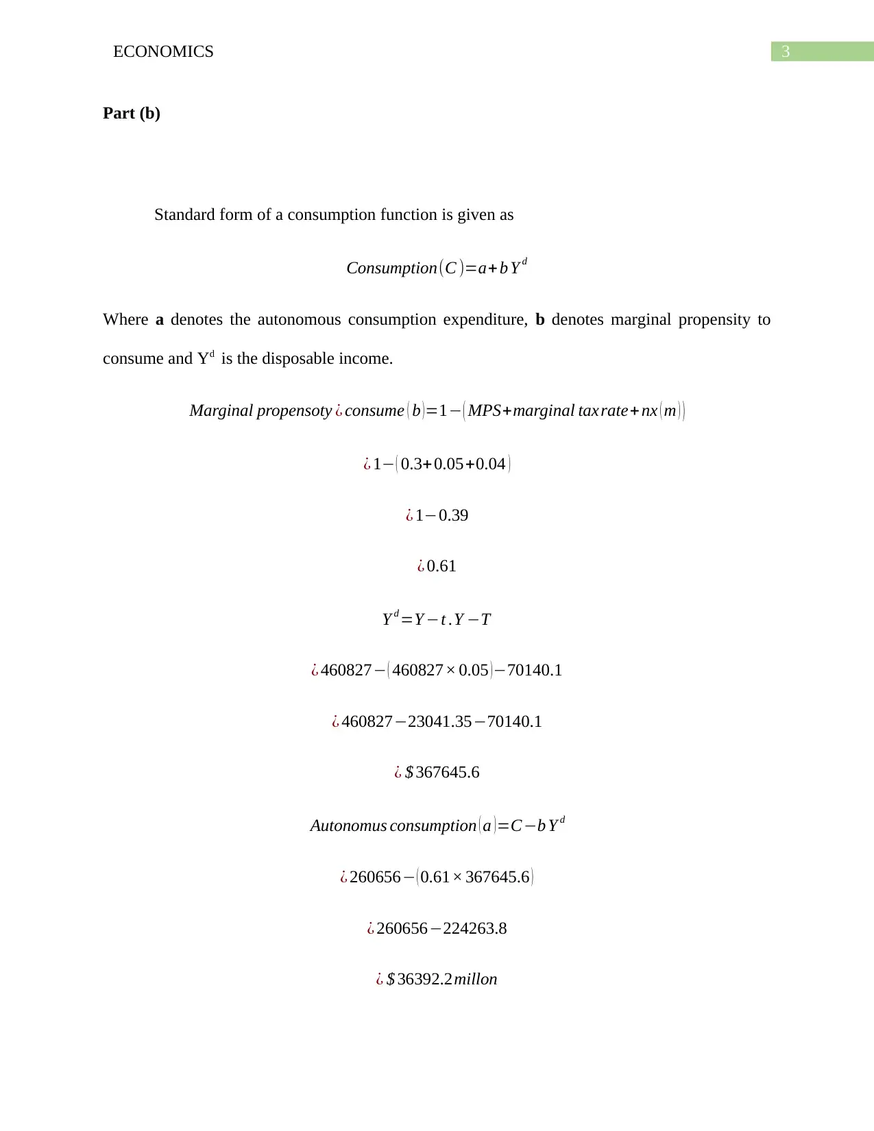
Consumption(C )=a+ b Y d
Where a denotes the autonomous consumption expenditure, b denotes marginal propensity to
consume and Yd is the disposable income.
Marginal propensoty ¿ consume ( b ) =1− ( MPS+marginal taxrate+ nx ( m ) )
¿ 1− ( 0.3+0.05+0.04 )
¿ 1−0.39
¿ 0.61
Y d =Y −t .Y −T
¿ 460827− ( 460827× 0.05 )−70140.1
¿ 460827−23041.35−70140.1
¿ $ 367645.6
Autonomus consumption ( a ) =C−b Y d
¿ 260656− ( 0.61× 367645.6 )
¿ 260656−224263.8
¿ $ 36392.2millon

4ECONOMICS
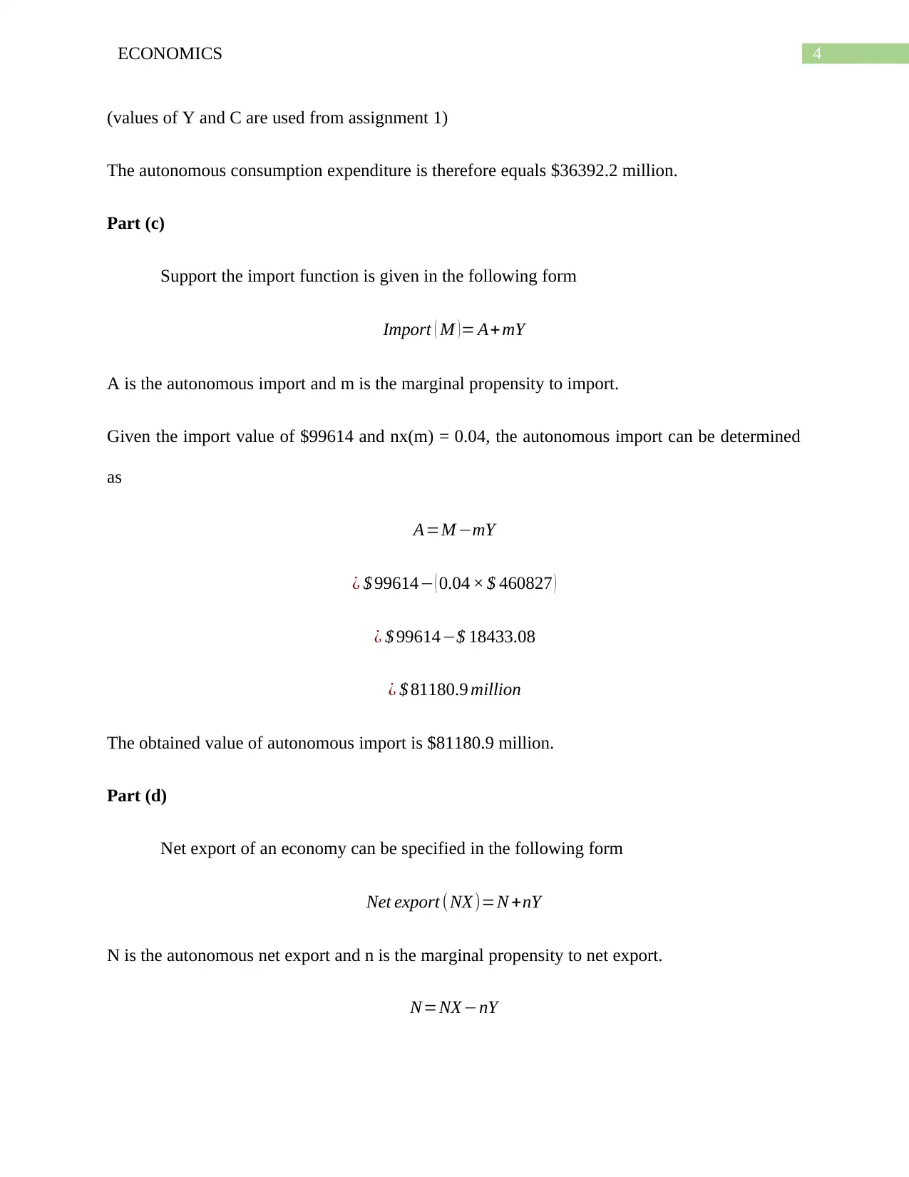
(values of Y and C are used from assignment 1)
The autonomous consumption expenditure is therefore equals $36392.2 million.
Part (c)
Support the import function is given in the following form
Import ( M ) = A+ mY
A is the autonomous import and m is the marginal propensity to import.
Given the import value of $99614 and nx(m) = 0.04, the autonomous import can be determined
as
A=M −mY
¿ $ 99614− ( 0.04 × $ 460827 )
¿ $ 99614−$ 18433.08
¿ $ 81180.9 million
The obtained value of autonomous import is $81180.9 million.
Part (d)
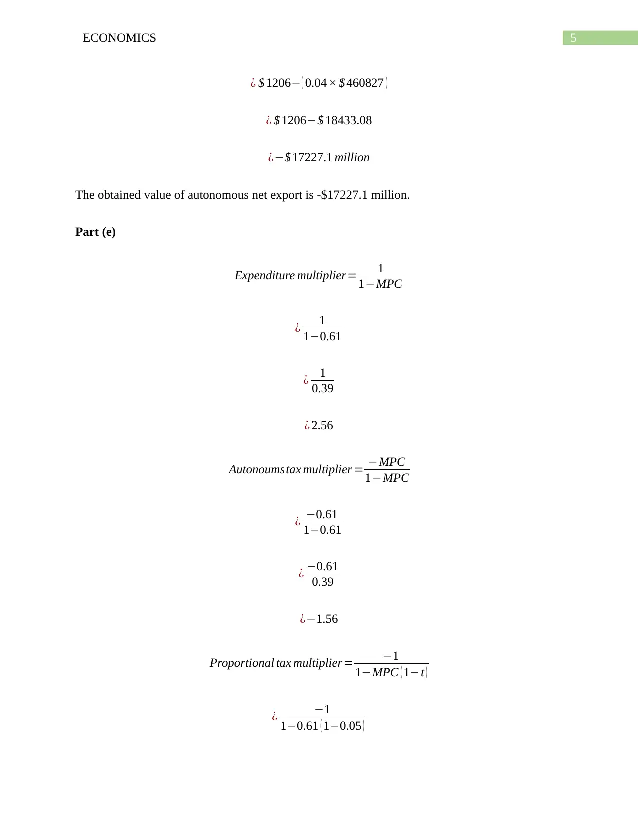
Net export of an economy can be specified in the following form
Net export (NX)=N +nY
N is the autonomous net export and n is the marginal propensity to net export.
N=NX −nY

5ECONOMICS
¿ $ 1206− ( 0.04 × $ 460827 )
¿ $ 1206−$ 18433.08
¿−$ 17227.1 million
The obtained value of autonomous net export is -$17227.1 million.
Part (e)
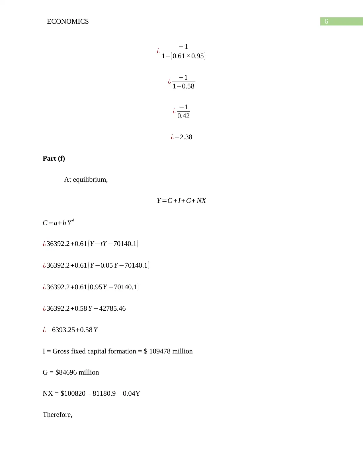
Expenditure multiplier= 1
1−MPC
¿ 1
1−0.61
¿ 1
0.39
¿ 2.56
Autonoumstax multiplier = −MPC
1−MPC
¿ −0.61
1−0.61
¿ −0.61
0.39
¿−1.56
Proportional tax multiplier= −1
1−MPC ( 1−t )
¿ −1
1−0.61 ( 1−0.05 )

6ECONOMICS
¿ −1
1− ( 0.61 ×0.95 )
¿ −1
1−0.58
¿ −1
0.42
¿−2.38
Part (f)
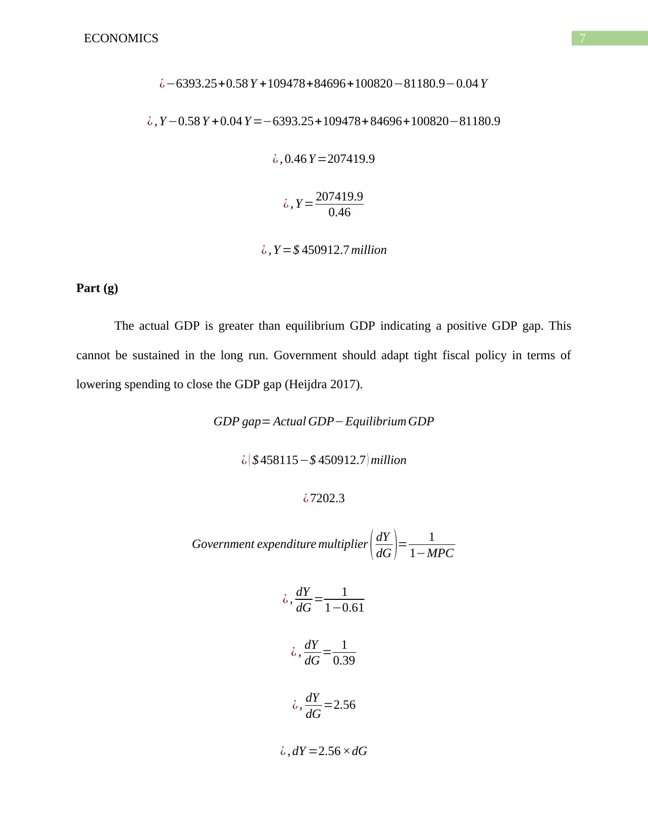
At equilibrium,
Y =C +I+ G+ NX
C=a+b Y d
¿ 36392.2+0.61 ( Y −tY −70140.1 )
¿ 36392.2+0.61 ( Y −0.05 Y −70140.1 )
¿ 36392.2+0.61 ( 0.95Y −70140.1 )
¿ 36392.2+0.58 Y −42785.46
¿−6393.25+0.58 Y
I = Gross fixed capital formation = $ 109478 million
G = $84696 million
NX = $100820 – 81180.9 – 0.04Y
Therefore,

7ECONOMICS
¿−6393.25+0.58 Y +109478+84696+100820−81180.9−0.04 Y
¿ , Y −0.58 Y +0.04 Y =−6393.25+109478+ 84696+100820−81180.9
¿ , 0.46 Y =207419.9
¿ , Y = 207419.9
0.46
¿ , Y =$ 450912.7 million
Part (g)
The actual GDP is greater than equilibrium GDP indicating a positive GDP gap. This
cannot be sustained in the long run. Government should adapt tight fiscal policy in terms of
lowering spending to close the GDP gap (Heijdra 2017).
GDP gap= Actual GDP−Equilibrium GDP
¿ ( $ 458115−$ 450912.7 ) million
¿ 7202.3
Government expenditure multiplier ( dY
dG )= 1
1−MPC
¿ , dY
dG = 1
1−0.61
¿ , dY
dG = 1
0.39
¿ , dY
dG =2.56
¿ , dY =2.56 ×dG

8ECONOMICS
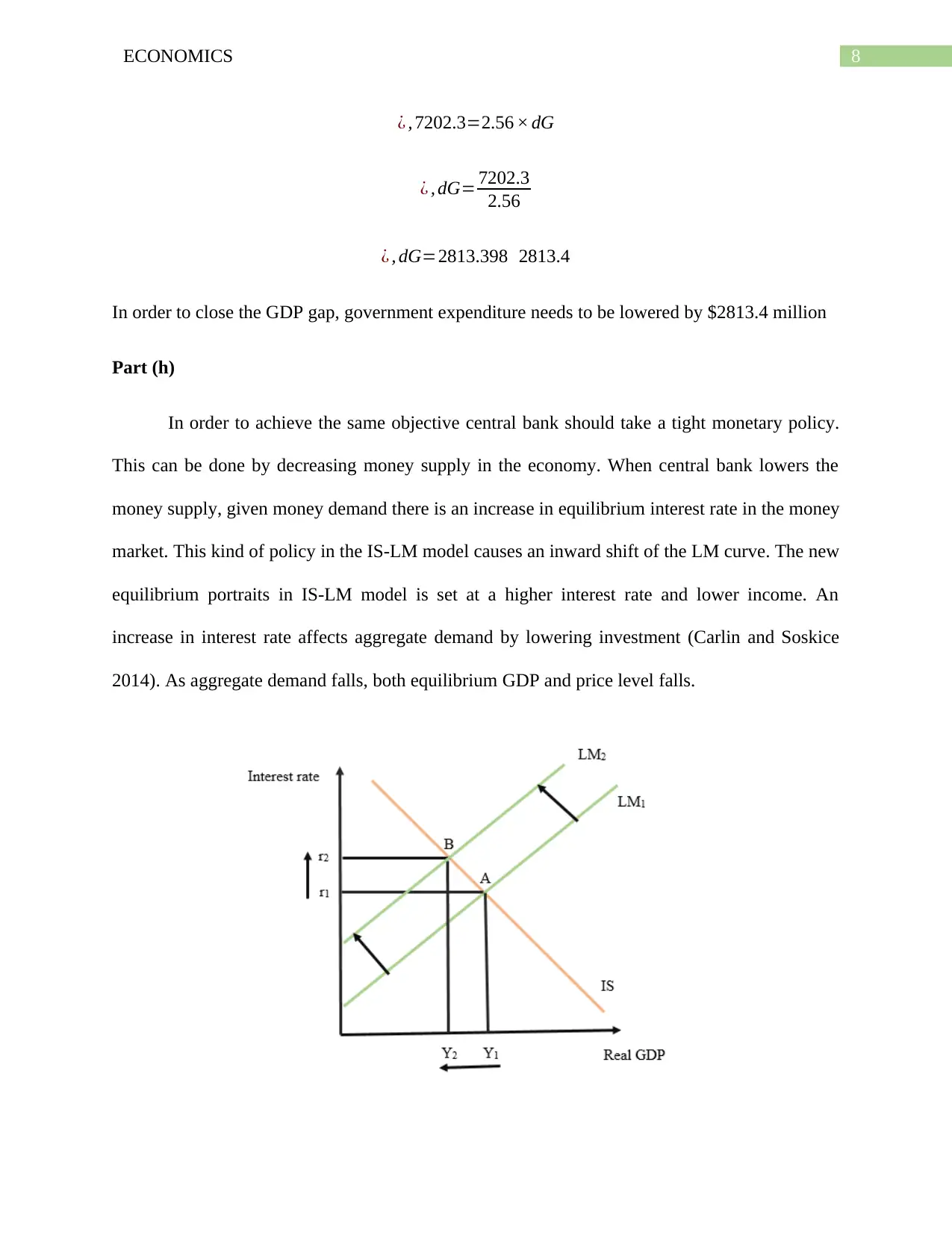
¿ , 7202.3=2.56 × dG
¿ , dG= 7202.3
2.56
¿ , dG=2813.398 2813.4
In order to close the GDP gap, government expenditure needs to be lowered by $2813.4 million
Part (h)
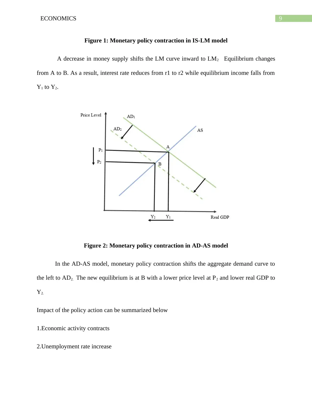
In order to achieve the same objective central bank should take a tight monetary policy.
This can be done by decreasing money supply in the economy. When central bank lowers the
money supply, given money demand there is an increase in equilibrium interest rate in the money
market. This kind of policy in the IS-LM model causes an inward shift of the LM curve. The new
equilibrium portraits in IS-LM model is set at a higher interest rate and lower income. An
increase in interest rate affects aggregate demand by lowering investment (Carlin and Soskice
2014). As aggregate demand falls, both equilibrium GDP and price level falls.

9ECONOMICS
Figure 1: Monetary policy contraction in IS-LM model
A decrease in money supply shifts the LM curve inward to LM2 Equilibrium changes
from A to B. As a result, interest rate reduces from r1 to r2 while equilibrium income falls from
Y1 to Y2.
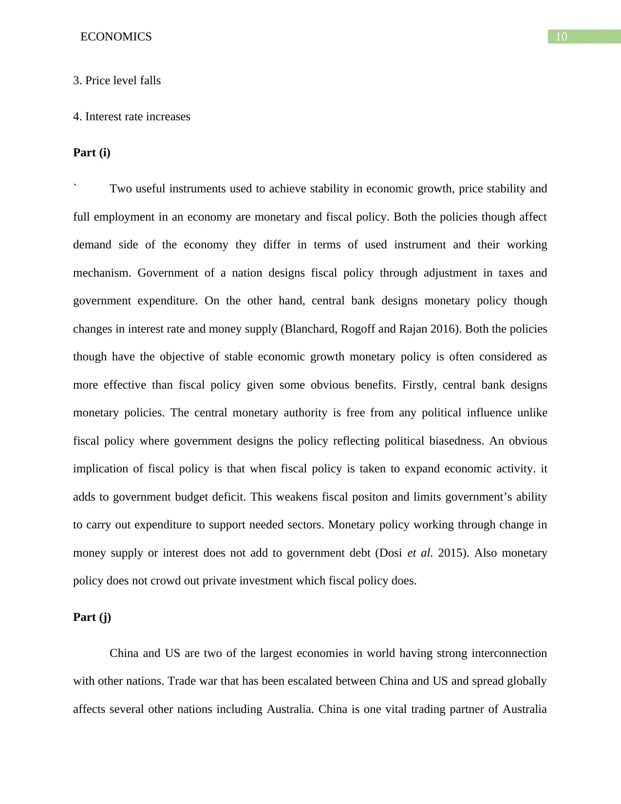
Figure 2: Monetary policy contraction in AD-AS model
In the AD-AS model, monetary policy contraction shifts the aggregate demand curve to
the left to AD2. The new equilibrium is at B with a lower price level at P2 and lower real GDP to
Y2.
Impact of the policy action can be summarized below
1.Economic activity contracts
2.Unemployment rate increase

10ECONOMICS
3. Price level falls
4. Interest rate increases
Part (i)
` Two useful instruments used to achieve stability in economic growth, price stability and
full employment in an economy are monetary and fiscal policy. Both the policies though affect
demand side of the economy they differ in terms of used instrument and their working
mechanism. Government of a nation designs fiscal policy through adjustment in taxes and
government expenditure. On the other hand, central bank designs monetary policy though
changes in interest rate and money supply (Blanchard, Rogoff and Rajan 2016). Both the policies
though have the objective of stable economic growth monetary policy is often considered as
more effective than fiscal policy given some obvious benefits. Firstly, central bank designs
monetary policies. The central monetary authority is free from any political influence unlike
fiscal policy where government designs the policy reflecting political biasedness. An obvious
implication of fiscal policy is that when fiscal policy is taken to expand economic activity. it
adds to government budget deficit. This weakens fiscal positon and limits government’s ability
to carry out expenditure to support needed sectors. Monetary policy working through change in
money supply or interest does not add to government debt (Dosi et al. 2015). Also monetary
policy does not crowd out private investment which fiscal policy does.
Part (j)
China and US are two of the largest economies in world having strong interconnection
with other nations. Trade war that has been escalated between China and US and spread globally
affects several other nations including Australia. China is one vital trading partner of Australia

11ECONOMICS
and the largest importing nation for Australian export. Trade war with China will lead to an
economic contraction of China reducing its ability to import from rest of the world. Australia
will thus face a decline in its export demand to the China’s market (Li, He and Lin 2018). The
lower export demand will cause Australian economy to contract as well. The contraction of
production activities will increase unemployment in the economy by lowering labor demand.
Another implication of trade escalation between China and US is the likely depreciation of
Australian dollar. The depreciated dollar will increase the price of imports adding to imported
inflation in the nation. Australia will suffer from a combined effect of lower economic growth,
higher unemployment, weak current and high inflation (Wang 2016). Trade war however is not
at all bad for the entire economy. Some sectors such as agriculture, steel and natural gas are
likely to get benefitted as the two of the largest nation imposes tariff on import from each other.

12ECONOMICS
List of references
Blanchard, M.O.J., Rogoff, M.K. and Rajan, R. eds., 2016. Progress and confusion: the state of
macroeconomic policy. International Monetary Fund.
Carlin, W. and Soskice, D.W., 2014. Macroeconomics: Institutions, instability, and the financial
system. Oxford University Press, USA.
Dosi, G., Fagiolo, G., Napoletano, M., Roventini, A. and Treibich, T., 2015. Fiscal and monetary
policies in complex evolving economies. Journal of Economic Dynamics and Control, 52,
pp.166-189.
Heijdra, B.J., 2017. Foundations of modern macroeconomics. Oxford university press.
Li, C., He, C. and Lin, C., 2018. Economic Impacts of the Possible China–US Trade
War. Emerging Markets Finance and Trade, 54(7), pp.1557-1577.
Wang, Y., 2016. Australia-China relations post 1949: Sixty years of trade and politics.
Routledge.