Microeconomics Assignment: Wine, Bicycles, and Production Costs
VerifiedAdded on 2023/01/17
|11
|1090
|82
Homework Assignment
AI Summary
This economics assignment solution addresses five short-answer questions covering core microeconomic principles. Question 1 analyzes production possibilities frontiers for wine production, including the impact of drought and market shifts. Question 2 explores price elasticity of demand for theme park tickets. Question 3 examines market equilibrium, the effects of taxation on the bicycle market, including consumer and producer surplus, and deadweight loss. Question 4 focuses on supply and demand analysis for bananas. Question 5 delves into cost analysis, including marginal product, fixed and variable costs, and the concept of diminishing returns to labor. The solutions provide detailed calculations, diagrams, and explanations to illustrate these economic concepts.
Running head: ECONOMICS
Economics
Name of the university
Name of the author
Author note
Economics
Name of the university
Name of the author
Author note
Paraphrase This Document
Need a fresh take? Get an instant paraphrase of this document with our AI Paraphraser
ECONOMICS
Answer 1
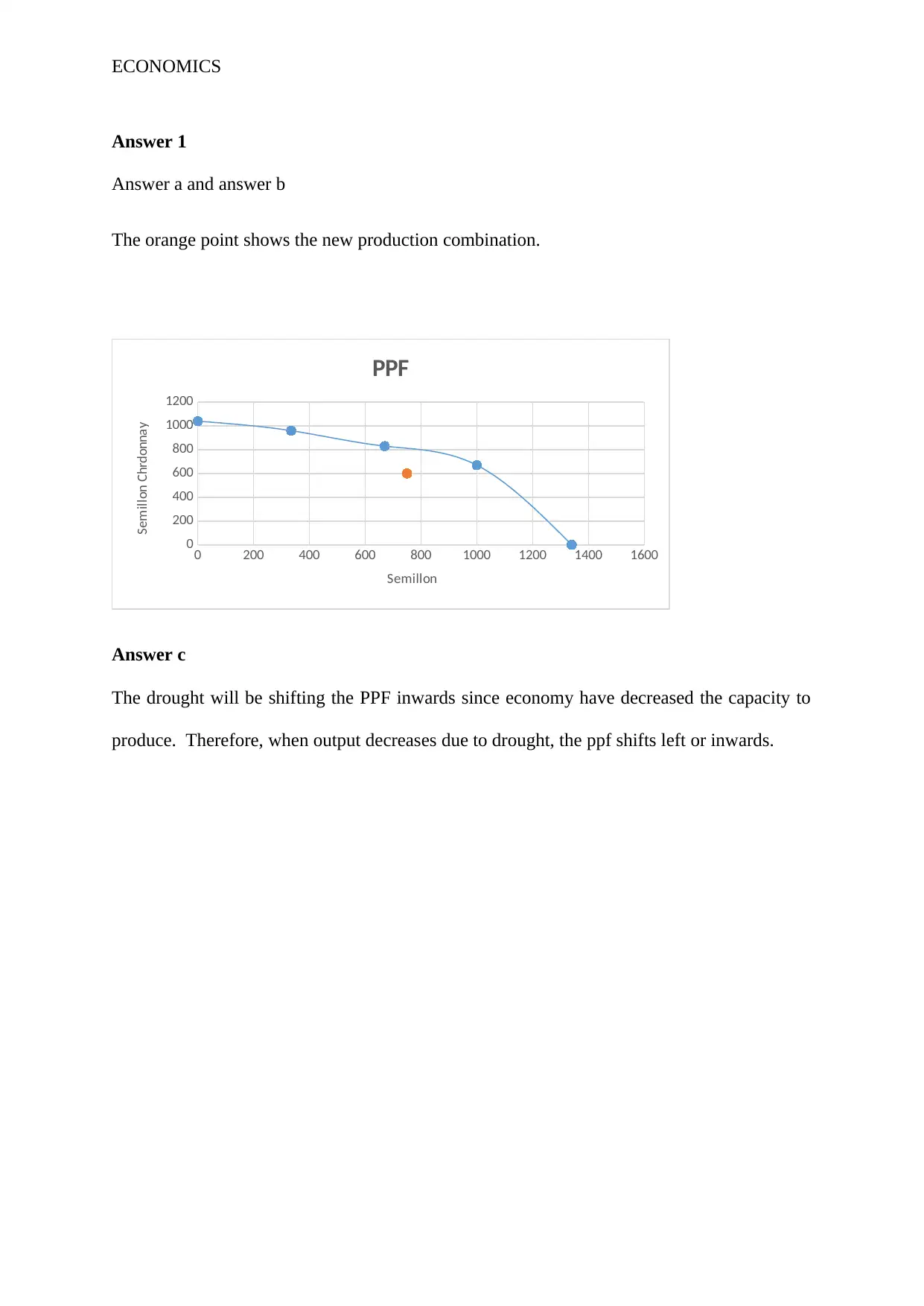
Answer a and answer b
The orange point shows the new production combination.
0 200 400 600 800 1000 1200 1400 1600
0
200
400
600
800
1000
1200
PPF
Semillon
Semillon Chrdonnay
Answer c
The drought will be shifting the PPF inwards since economy have decreased the capacity to
produce. Therefore, when output decreases due to drought, the ppf shifts left or inwards.
D
D1
D
P
S1
S2
ECONOMICS
Answer d
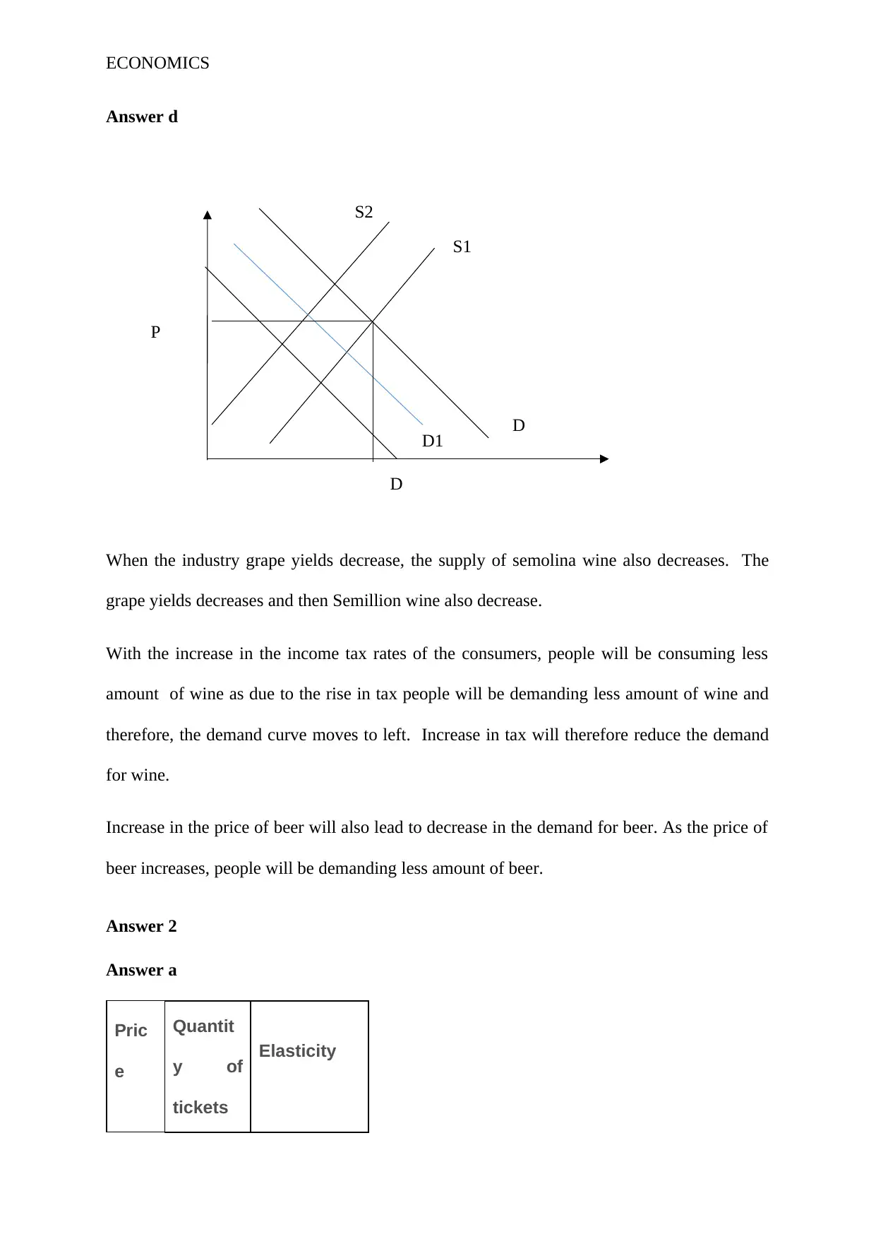
When the industry grape yields decrease, the supply of semolina wine also decreases. The
grape yields decreases and then Semillion wine also decrease.
With the increase in the income tax rates of the consumers, people will be consuming less
amount of wine as due to the rise in tax people will be demanding less amount of wine and
therefore, the demand curve moves to left. Increase in tax will therefore reduce the demand
for wine.
Increase in the price of beer will also lead to decrease in the demand for beer. As the price of
beer increases, people will be demanding less amount of beer.
Answer 2
Answer a
Pric
e
Quantit
y of
tickets
Elasticity
⊘ This is a preview!⊘
Do you want full access?
Subscribe today to unlock all pages.

Trusted by 1+ million students worldwide
ECONOMICS
sold per
day
0 1200 --
20 1050 0
40 900 -0.14285714
60 750 -0.33333333
80 600 -0.6
100 450 -1
120 300 -1.66666667
140 150 -3
160 0 Infinity
Answer b
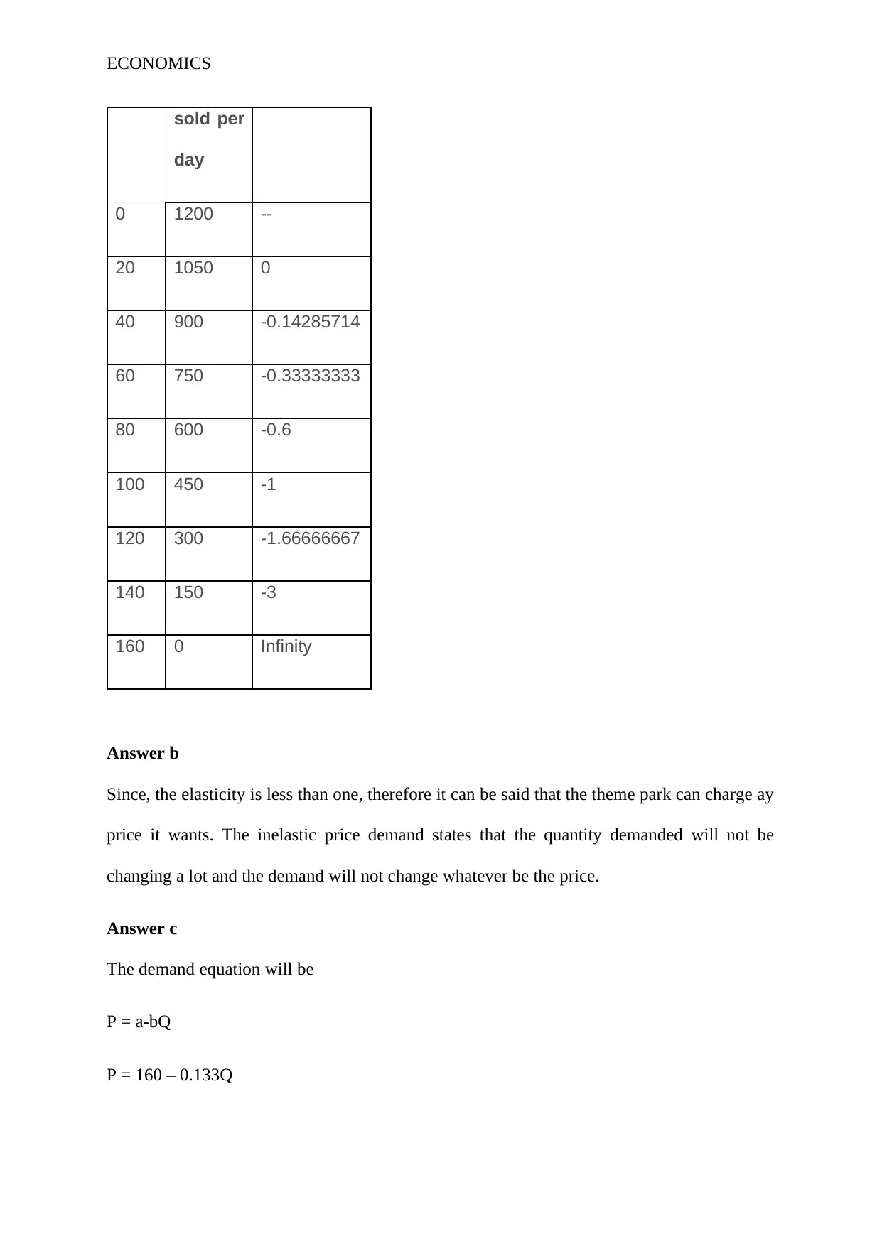
Since, the elasticity is less than one, therefore it can be said that the theme park can charge ay
price it wants. The inelastic price demand states that the quantity demanded will not be
changing a lot and the demand will not change whatever be the price.
Answer c
The demand equation will be
P = a-bQ
P = 160 – 0.133Q
Paraphrase This Document
Need a fresh take? Get an instant paraphrase of this document with our AI Paraphraser
ECONOMICS
Answer d
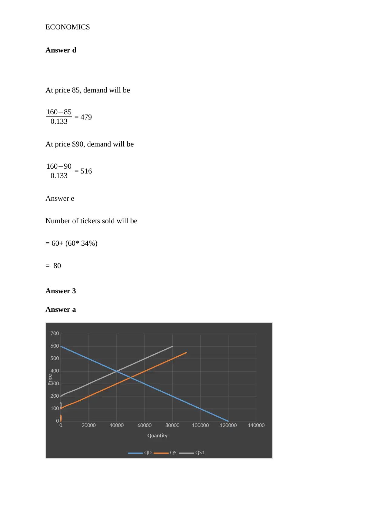
At price 85, demand will be
160−85
0.133 = 479
At price $90, demand will be
160−90
0.133 = 516
Answer e
Number of tickets sold will be
= 60+ (60* 34%)
= 80
Answer 3
Answer a
0 20000 40000 60000 80000 100000 120000 140000
0
100
200
300
400
500
600
700
QD QS QS1
Quantity
Price
Answer d
At price 85, demand will be
160−85
0.133 = 479
At price $90, demand will be
160−90
0.133 = 516
Answer e
Number of tickets sold will be
= 60+ (60* 34%)
= 80
Answer 3
Answer a
0 20000 40000 60000 80000 100000 120000 140000
0
100
200
300
400
500
600
700
QD QS QS1
Quantity
Price
ECONOMICS
Answer b
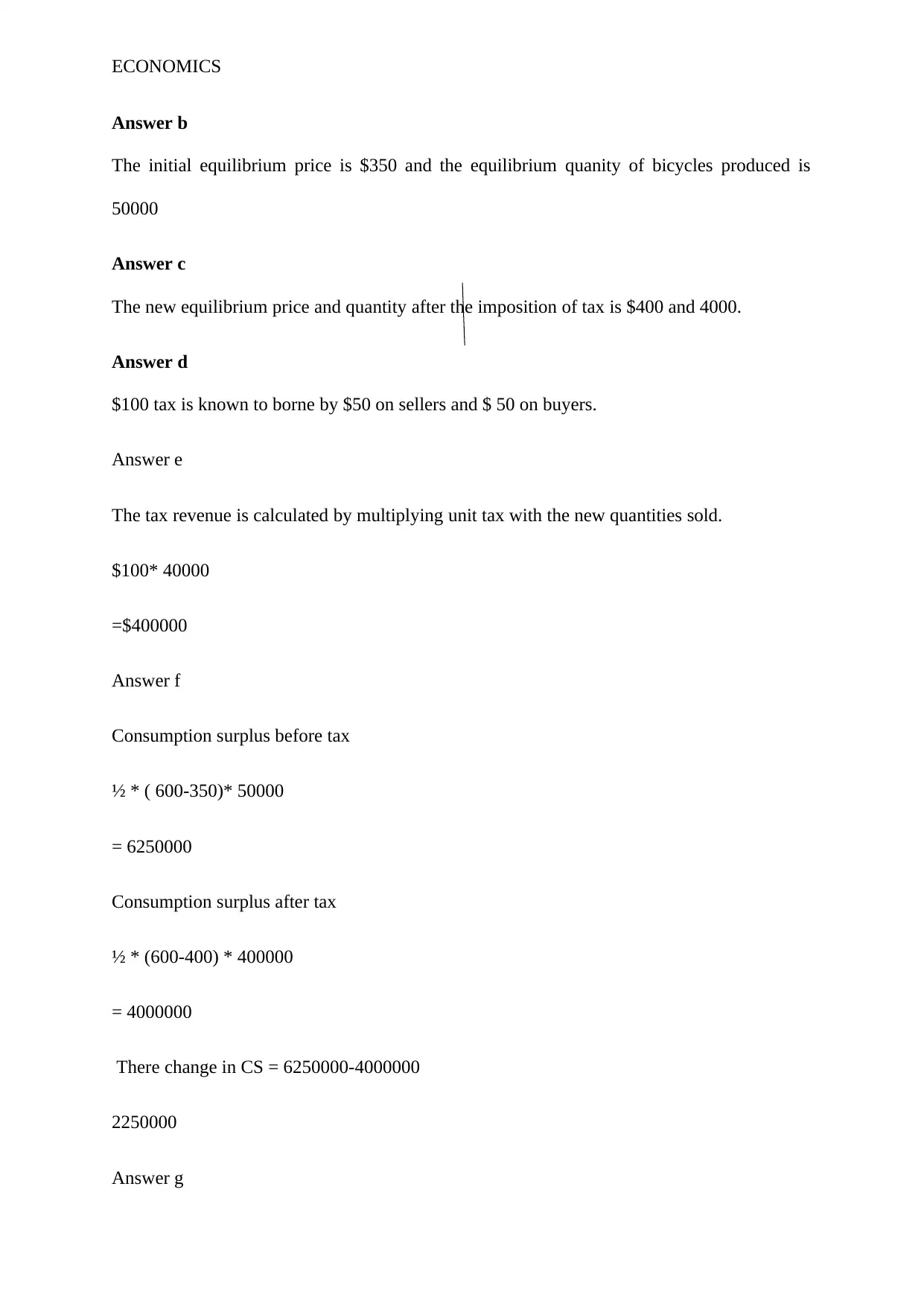
The initial equilibrium price is $350 and the equilibrium quanity of bicycles produced is
50000
Answer c
The new equilibrium price and quantity after the imposition of tax is $400 and 4000.
Answer d
$100 tax is known to borne by $50 on sellers and $ 50 on buyers.
Answer e
The tax revenue is calculated by multiplying unit tax with the new quantities sold.
$100* 40000
=$400000
Answer f
Consumption surplus before tax
½ * ( 600-350)* 50000
= 6250000
Consumption surplus after tax
½ * (600-400) * 400000
= 4000000
There change in CS = 6250000-4000000
2250000
Answer g
⊘ This is a preview!⊘
Do you want full access?
Subscribe today to unlock all pages.

Trusted by 1+ million students worldwide
ECONOMICS
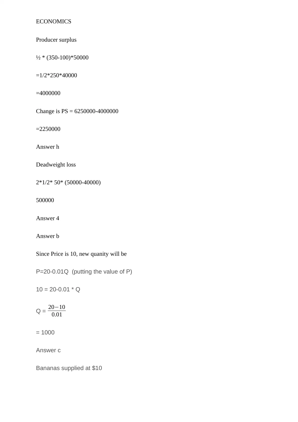
Producer surplus
½ * (350-100)*50000
=1/2*250*40000
=4000000
Change is PS = 6250000-4000000
=2250000
Answer h
Deadweight loss
2*1/2* 50* (50000-40000)
500000
Answer 4
Answer b
Since Price is 10, new quanity will be
P=20-0.01Q (putting the value of P)
10 = 20-0.01 * Q
Q = 20−10
0.01
= 1000
Answer c
Bananas supplied at $10
Paraphrase This Document
Need a fresh take? Get an instant paraphrase of this document with our AI Paraphraser
ECONOMICS
P=2+0.02Q
Q = 10−2
0.02
= 400
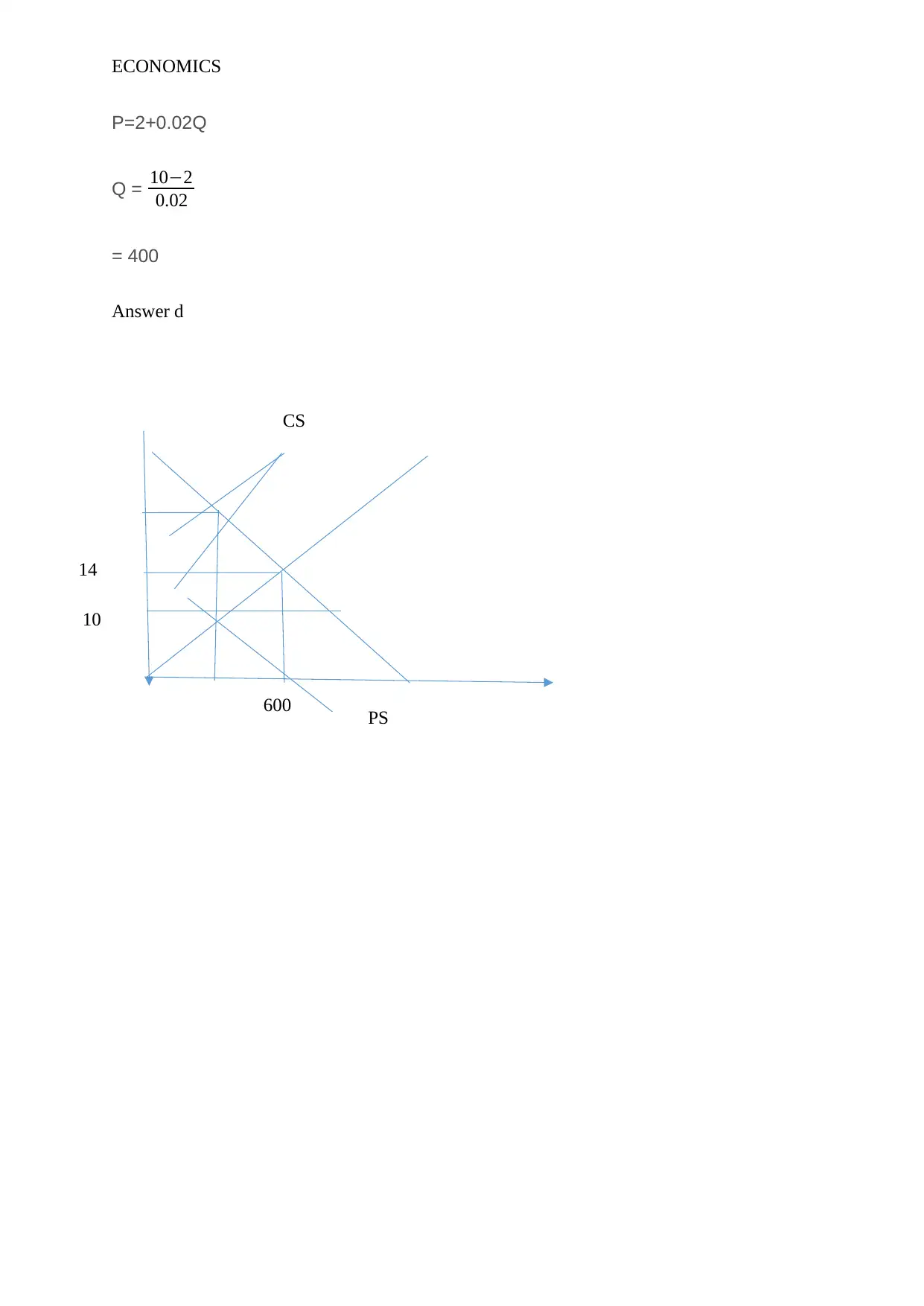
Answer d
14
600
10
CS
PS
P=2+0.02Q
Q = 10−2
0.02
= 400
Answer d
14
600
10
CS
PS
ECONOMICS
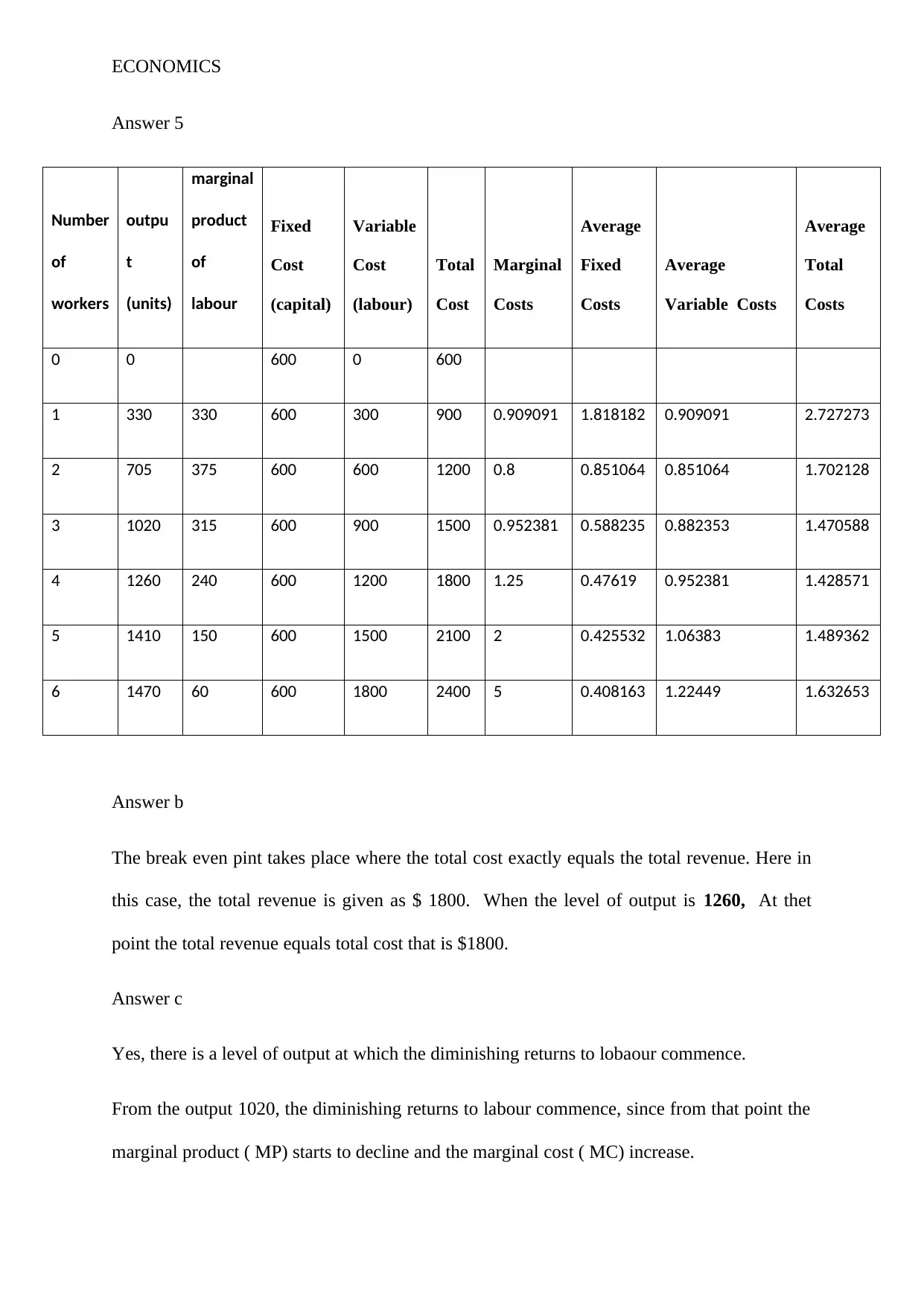
Answer 5
Number
of
workers
outpu
t
(units)
marginal
product
of
labour
Fixed
Cost
(capital)
Variable
Cost
(labour)
Total
Cost
Marginal
Costs
Average
Fixed
Costs
Average
Variable Costs
Average
Total
Costs
0 0 600 0 600
1 330 330 600 300 900 0.909091 1.818182 0.909091 2.727273
2 705 375 600 600 1200 0.8 0.851064 0.851064 1.702128
3 1020 315 600 900 1500 0.952381 0.588235 0.882353 1.470588
4 1260 240 600 1200 1800 1.25 0.47619 0.952381 1.428571
5 1410 150 600 1500 2100 2 0.425532 1.06383 1.489362
6 1470 60 600 1800 2400 5 0.408163 1.22449 1.632653
Answer b
The break even pint takes place where the total cost exactly equals the total revenue. Here in
this case, the total revenue is given as $ 1800. When the level of output is 1260, At thet
point the total revenue equals total cost that is $1800.
Answer c
Yes, there is a level of output at which the diminishing returns to lobaour commence.
From the output 1020, the diminishing returns to labour commence, since from that point the
marginal product ( MP) starts to decline and the marginal cost ( MC) increase.
⊘ This is a preview!⊘
Do you want full access?
Subscribe today to unlock all pages.

Trusted by 1+ million students worldwide
ECONOMICS
Answer d
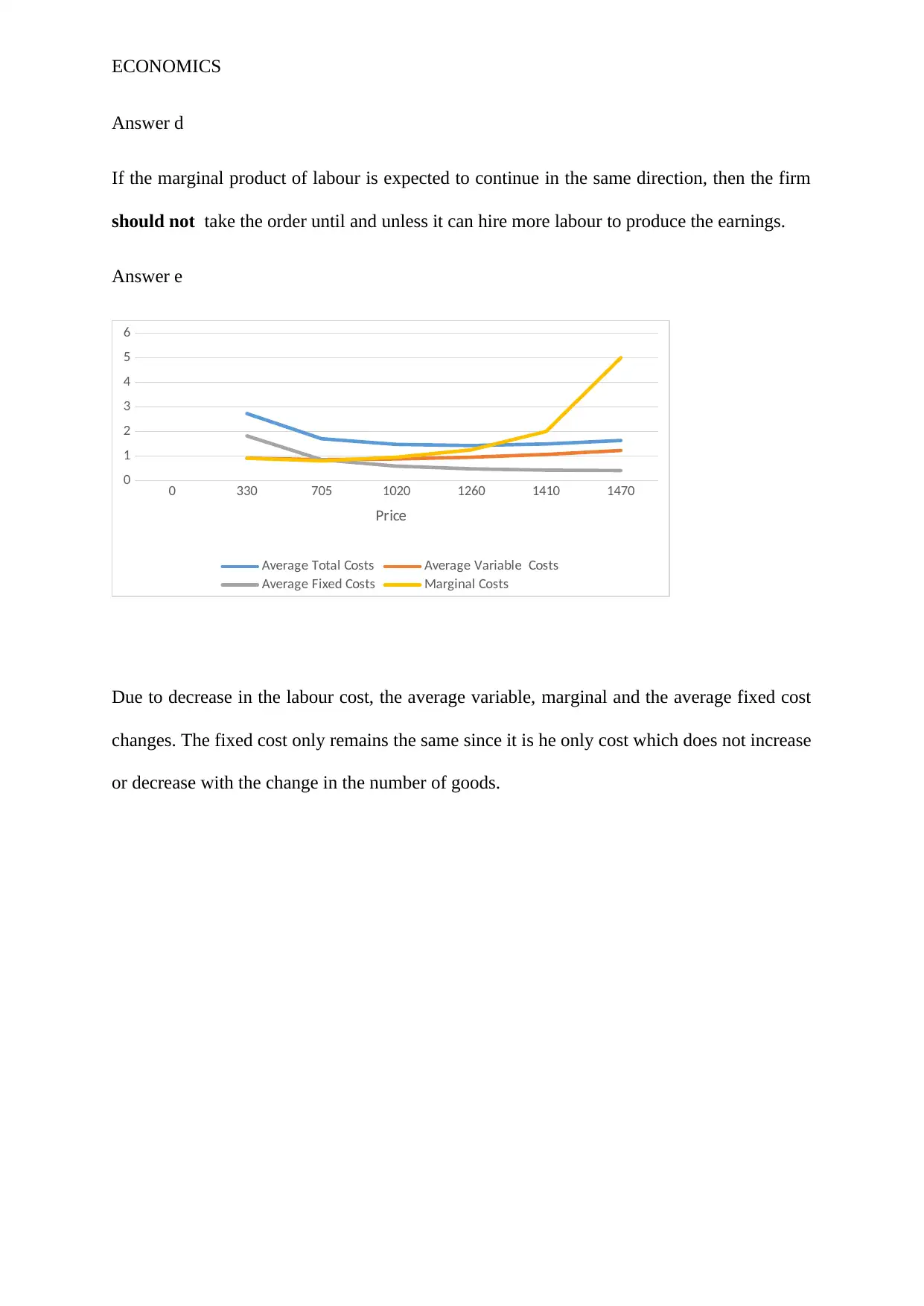
If the marginal product of labour is expected to continue in the same direction, then the firm
should not take the order until and unless it can hire more labour to produce the earnings.
Answer e
0 330 705 1020 1260 1410 1470
0
1
2
3
4
5
6
Average Total Costs Average Variable Costs
Average Fixed Costs Marginal Costs
Price
Due to decrease in the labour cost, the average variable, marginal and the average fixed cost
changes. The fixed cost only remains the same since it is he only cost which does not increase
or decrease with the change in the number of goods.
Paraphrase This Document
Need a fresh take? Get an instant paraphrase of this document with our AI Paraphraser
ECONOMICS
Reference list
Bade, R., & Parkin, M. (2015). Foundations of microeconomics. Pearson.
Bauer, M. J. R. (2018). Principles of microeconomics.
Baumol, W. J., & Blinder, A. S. (2015). Microeconomics: Principles and policy. Nelson
Education.
Cowen, T., & Tabarrok, A. (2015). Modern principles of microeconomics. Macmillan
International Higher Education.
Friedman, L. S. (2017). The microeconomics of public policy analysis. Princeton University
Press.
Iossa, E., & Martimort, D. (2015). The simple microeconomics of public‐private partnerships.
Journal of Public Economic Theory, 17(1), 4-48.
Khalil, F., Lawarree, J., & Scott, T. J. (2018). Applied Microeconomics.
Kreps, D. M. (2019). Microeconomics for managers. Princeton University Press.
1 out of 11
Your All-in-One AI-Powered Toolkit for Academic Success.
+13062052269
info@desklib.com
Available 24*7 on WhatsApp / Email
![[object Object]](/_next/static/media/star-bottom.7253800d.svg)
Unlock your academic potential
Copyright © 2020–2026 A2Z Services. All Rights Reserved. Developed and managed by ZUCOL.
