Macroeconomics: Aggregate Demand & Supply

This macroeconomics assignment examines the effects of global trade slowdowns and housing price declines on a national economy. It uses graphs to illustrate how shifts in aggregate demand (AD) and aggregate supply (AS) lead to changes in output (GDP) and price levels. The analysis covers the consequences of reduced export earnings due to slower world trade and the contractionary effect of falling house prices on investment and aggregate supply.

Running Head: ECONOMICS FOR BUSINESS ENVIRONMENT
Economics for Business Environment
Name of the Student
Name of the University
Author note

1ECONOMICS FOR BUSINESS ENVIRONMENT
Table of Contents
Answer 1..........................................................................................................................................2
Answer a......................................................................................................................................2
Answer b......................................................................................................................................4
Answer 2..........................................................................................................................................5
Answer 3..........................................................................................................................................7
References........................................................................................................................................9

2ECONOMICS FOR BUSINESS ENVIRONMENT
Answer 1
Answer a
In an economy, aggregate demand is the total goods and services demanded in a given
period. It shows the relation between level of prices and the goods and services that a country
produces domestically and captures consumption made by consumers, government, business and
foreigners. An inverse relation exists between price aggregate demands. That means as price
increases demand by different economic agents decreases making the demand curve downward
sloping from left to right. The aggregate supply on the other hand captures the relation between
price level and total goods and services produced by all the suppliers in a nation (Hubbard and
O'brien 2015).. An increase in the price level encourages suppliers to supply more. The positive
relation between price and quantity supplied makes the aggregate supply curve positively sloped.
Equilibrium in an economy is determined from intersection of aggregate demand and aggregate
supply curve. There are factors that cause a change in aggregate demand and aggregate supply
curve. Accordingly, output and price level change, causing change in other macroeconomic
variables (Benhabib, Wang and Wen 2015).
Metals consuming economy

3ECONOMICS FOR BUSINESS ENVIRONMENT
Figure 2: Effect of price increase in metal producing economy
(Source: as created by Author)
The aggregate supply and aggregate demand together determine macroeconomic
equilibrium. GDP and price level are the two most important economic variables. Figure 2
portraits the scenario of a metal consuming economy. The downward sloping curve AD is the
aggregate demand curve while the upward sloping curve AS is the aggregate supply curve. The
economic equilibrium is at point E. Consequently, Y* is the total output and price level
prevailing in economy is given as P*. Now, when price of non-precious metals rises then the
direct effect is on the aggregate demand of economic agents (Bernanke, Antonovics and Frank
2015). Because of a high price, they now demand a less amount of metal. This reduces the
aggregate demand of the economy. The decline in aggregate demand causes an inward shift in
aggregate demand curve. The aggregate demand curve shifts from AD to AD1. The new
aggregate demand curve with given aggregate supply changes the equilibrium from E to E1.

4ECONOMICS FOR BUSINESS ENVIRONMENT
Corresponding to the new equilibrium real GDP declines from Y* to Y1. As the output and
demand contract the price level reduces from P* to P1 causing a deflation in the economy.
Answer b
Metals producing economy
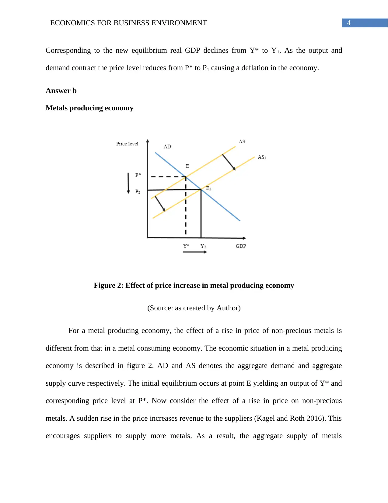
Figure 2: Effect of price increase in metal producing economy
(Source: as created by Author)
For a metal producing economy, the effect of a rise in price of non-precious metals is
different from that in a metal consuming economy. The economic situation in a metal producing
economy is described in figure 2. AD and AS denotes the aggregate demand and aggregate
supply curve respectively. The initial equilibrium occurs at point E yielding an output of Y* and
corresponding price level at P*. Now consider the effect of a rise in price on non-precious
metals. A sudden rise in the price increases revenue to the suppliers (Kagel and Roth 2016). This
encourages suppliers to supply more metals. As a result, the aggregate supply of metals

5ECONOMICS FOR BUSINESS ENVIRONMENT
increases. This is seen from an outward shift of aggregate supply curve. The supply curve shifts
from earlier AS to AS1. In correspondence to the new supply curve, a new equilibrium is
achieved at E2. As it is a metal producing economy, the increased supply of metal will raise the
total output. The GDP increases from Y* to Y2. The excess supply in the economy reduces the
overall price level or inflation. This means at the new equilibrium E2, output expands with a
lower level of prices (Challe et al. 2017). The new price at P2.
Answer 2
Aggregate demand is obtained as a sum of consumption expenditure, investment
expenditure, government expenditure and net expenditure. Change in any one of this components
causes a change in aggregate demand and hence, national output and level of prices (Mankiw
2014).
AD = C + I +G + (X – M)
C: Consumption
I: Investment
G: Government Expenditure
X: Export
M: Import
A slow-down of growth of world trade affects the aggregate demand. This is shown is the
following figure.

6ECONOMICS FOR BUSINESS ENVIRONMENT
Figure 3: Effect of a slowdown of world trade
(Source: as created by Author)
The aggregate demand and aggregate supply curve in the economy is given as AD and
AS respectively. The macroeconomic equilibrium is given as e. The output and price at the
equilibrium are Ye and Pe respectively. When there is slow-down in the growth of world trade,
then export earnings will be reduced. With contraction in global trade, exports and imports
contract and net export declines. As foreign demand is one source of aggregate demand,
aggregate demand in the economy decreases as shown by a leftward shift of the AD curve (Uribe
and Schmitt-Grohé 2017). The AD curve shifts left from AD to AD2. As a result, the economy as
whole contracts with a decline in output level to Y’ and that of the price level to P’.

7ECONOMICS FOR BUSINESS ENVIRONMENT
Answer 3
Figure 4: Effect of a fall in housing prices
(Source: as created by Author)
A major fall in house prices affect the aggregate supply in the economy. A positive
relation exists between price and aggregate supply. Initially the economy is in an equilibrium
state at point e. The price level is at Pe and correspond output is at Ye. Now, a falling house
price causes a decline in return to housing investment. Housing market being one of the
important sector of the economy will contract. The supply of housing and hence, aggregate
supply reduces. The decline in aggregate supply is shown from a leftward shift of the aggregate
supply curve (Currie, Nobay and Peel 2015). The aggregate supply curve shifts from AS to AS1.
The new equilibrium is at e2. As housing market contracts, the economy suffers from a shortage
of supply. The real GDP decreases from Ye to Y”. The economy wide shortage of supply push

8ECONOMICS FOR BUSINESS ENVIRONMENT
up economic price level and brings an inflationary pressure. Accordingly, the price level
increases from Pe to P”.

9ECONOMICS FOR BUSINESS ENVIRONMENT
References
Benhabib, J., Wang, P. and Wen, Y., 2015. Sentiments and aggregate demand
fluctuations. Econometrica, 83(2), pp.549-585.
Bernanke, B., Antonovics, K. and Frank, R., 2015. Principles of macroeconomics. McGraw-Hill
Higher Education.
Challe, E., Matheron, J., Ragot, X. and Rubio‐Ramirez, J.F., 2017. Precautionary saving and
aggregate demand. Quantitative Economics, 8(2), pp.435-478.
Currie, D., Nobay, R. and Peel, D., 2015. Macroeconomic analysis: essays in macroeconomics
and econometrics (Vol. 5). Routledge.
Hubbard, G. P. and O'brien, A. P. , 2015. Macroeconomics. Pearson Education.
Kagel, J.H. and Roth, A.E., 2016. Macroeconomics: A survey of laboratory research. Princeton
University Press.
Mankiw, N.G., 2014. Principles of macroeconomics. Cengage Learning.
Uribe, M. and Schmitt-Grohé, S., 2017. Open economy macroeconomics. Princeton University
Press.