EECS 152B Assignment 4: Implementing Sample Rate Conversion in MATLAB
VerifiedAdded on 2023/04/21
|30
|3489
|56
Homework Assignment
AI Summary
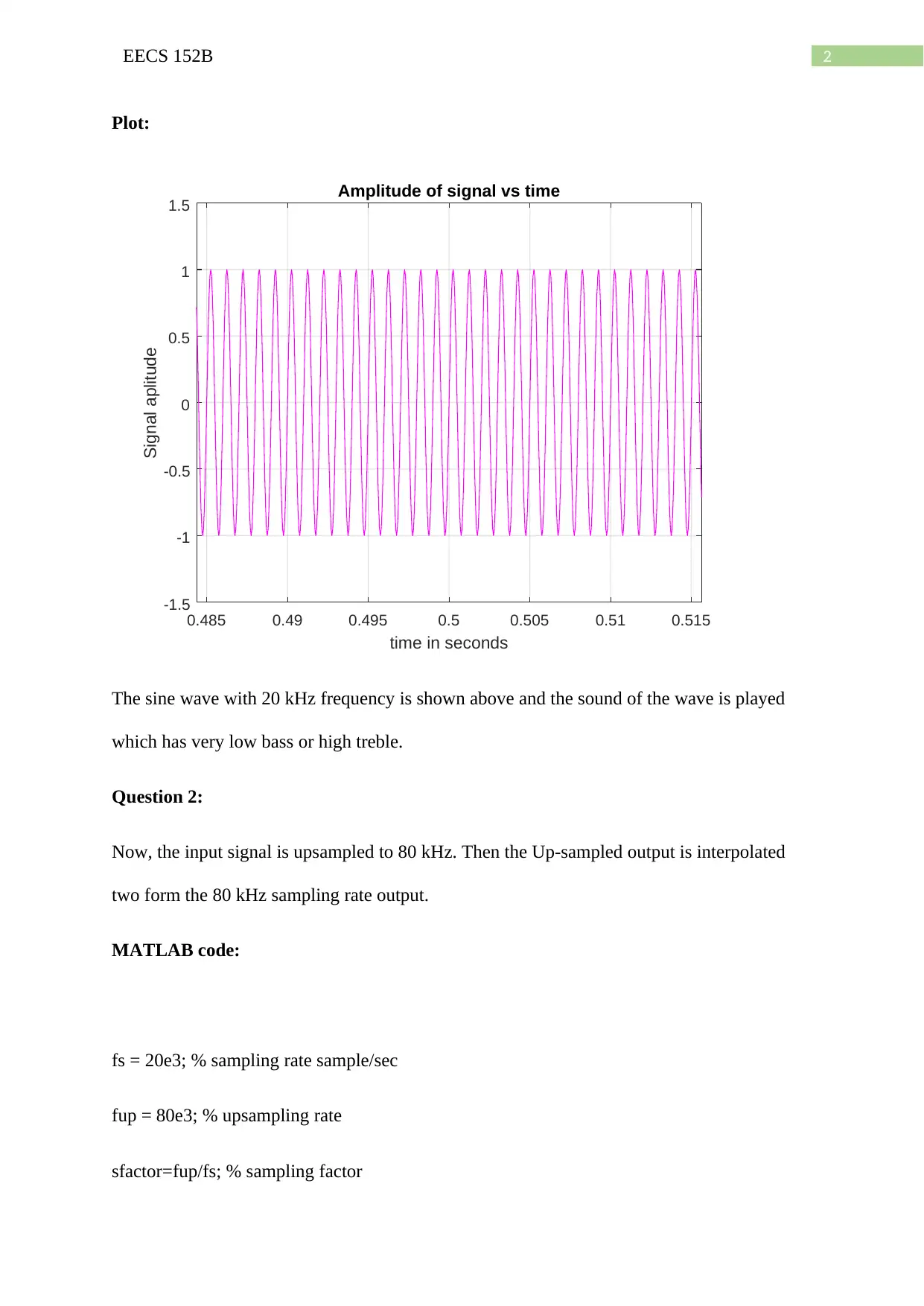
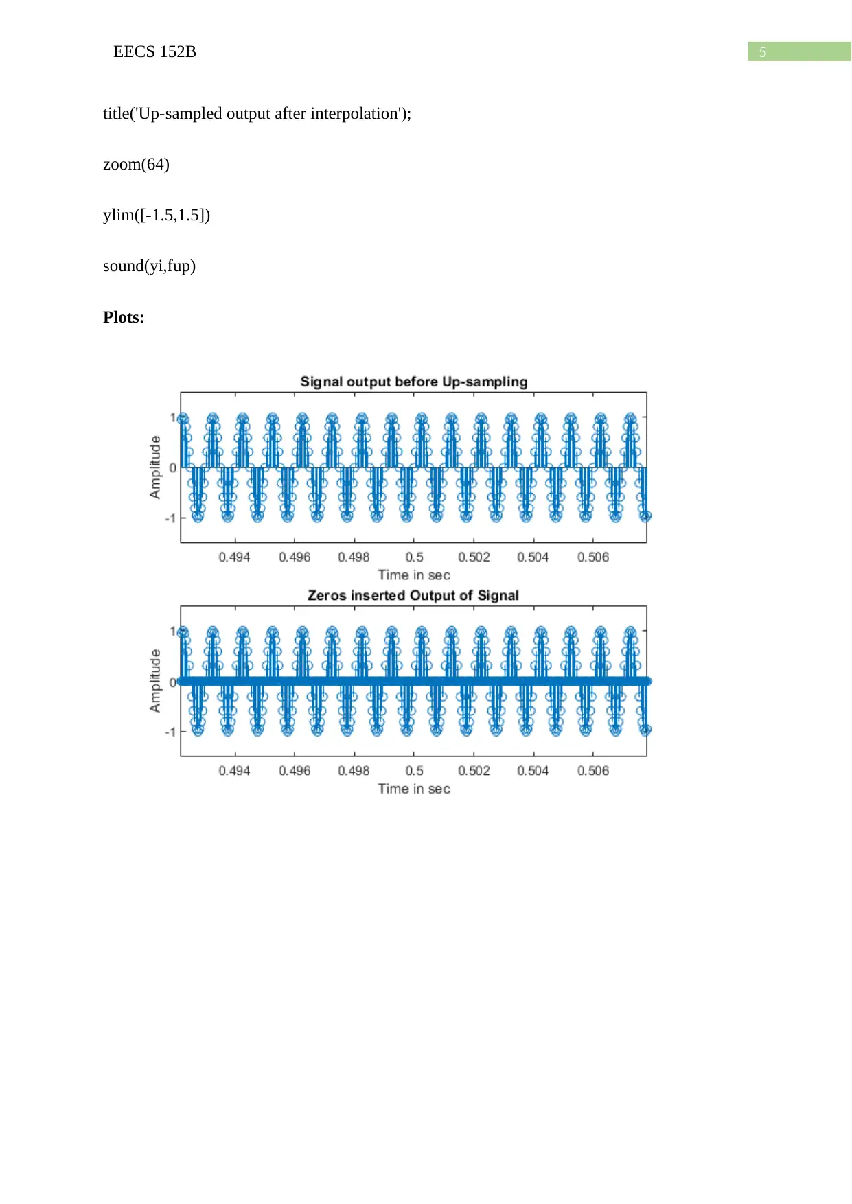
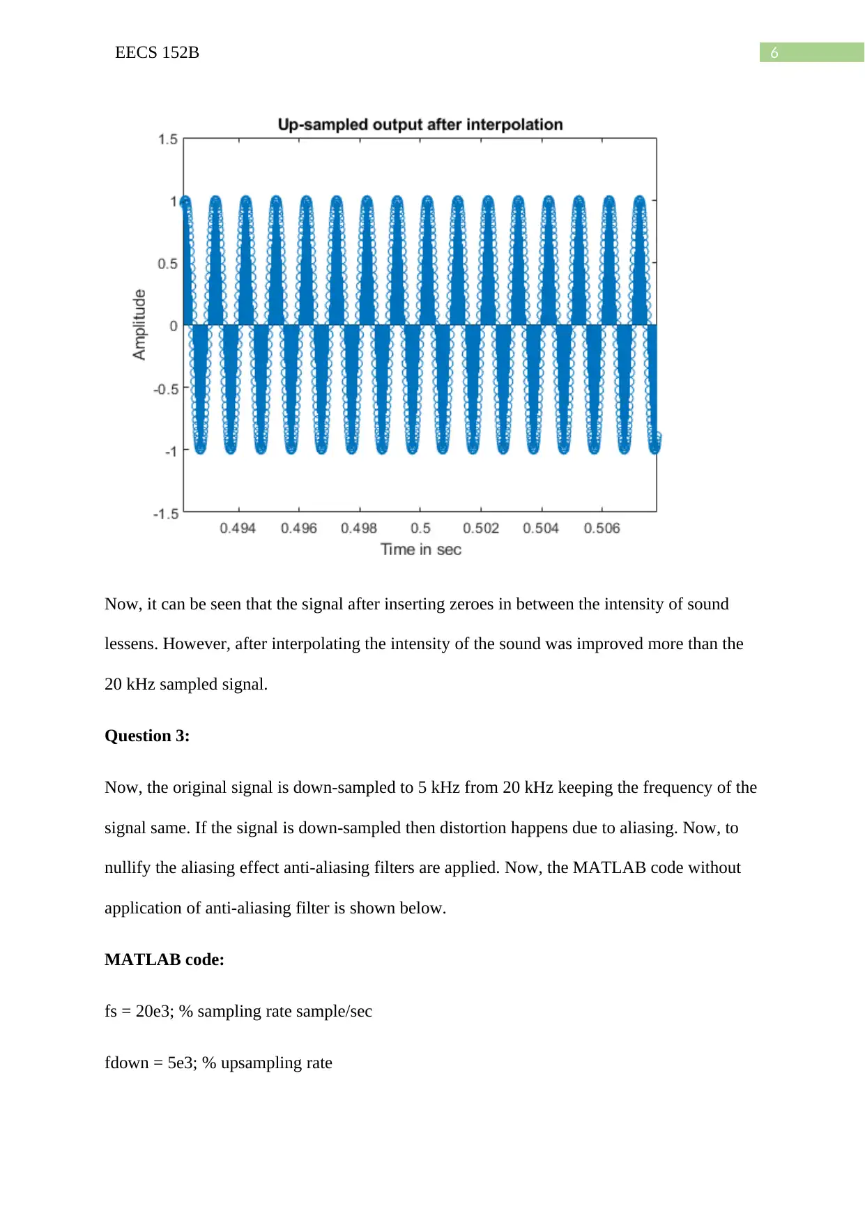
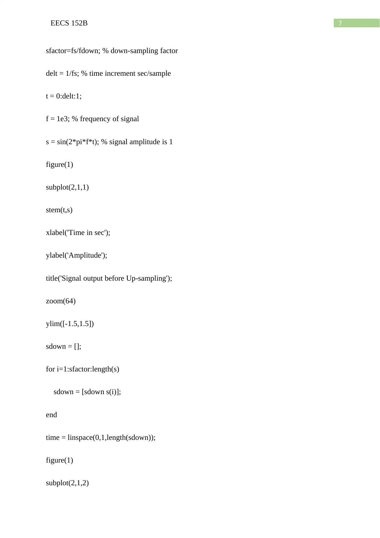
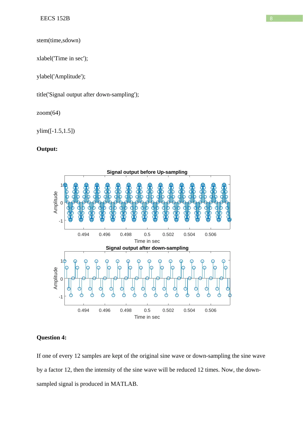
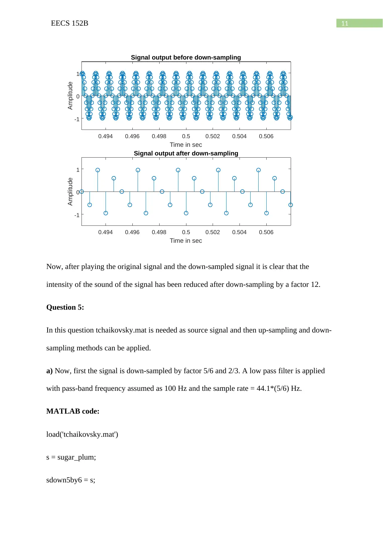
This assignment solution for EECS 152B, focuses on sample rate conversion techniques using MATLAB. It begins by generating and analyzing a 1000 Hz sine wave sampled at 20 kHz, playing the sound, and observing the effect. The solution then addresses upsampling to 80 kHz, exploring zero insertion and interpolation, and comparing the sound before and after each process. Next, the assignment investigates downsampling to 5 kHz and the necessity of anti-aliasing filters to mitigate aliasing effects. Further, the solution examines downsampling by a factor of 12 and its impact on signal intensity. Finally, it uses the 'tchaikovsky.mat' file to explore downsampling with factors 5/6 and 2/3, applying low-pass filters, and then downsampling with factors 1/2, 1/3 and 1/6. The solution also covers upsampling with factors 3/2, 9/2, and 21/2, applying low-pass filters and linear interpolator filters to remove aliasing effects and comparing the outcomes. The assignment demonstrates the effects of different rate conversion techniques on signal quality and the importance of filtering.
1 out of 30



![[object Object]](/_next/static/media/star-bottom.7253800d.svg)