Electronic Dynamics and controls Case Study 2022
VerifiedAdded on 2022/10/01
|24
|2104
|18
AI Summary
Contribute Materials
Your contribution can guide someone’s learning journey. Share your
documents today.
Electronics
Dynamics and controls
Position and Speed Control of a 1 – DOF Torsional Mechanical System
Student Name –
Student ID -
Dynamics and controls
Position and Speed Control of a 1 – DOF Torsional Mechanical System
Student Name –
Student ID -
Secure Best Marks with AI Grader
Need help grading? Try our AI Grader for instant feedback on your assignments.
Contents
Introduction...........................................................................................................................................2
Aim :......................................................................................................................................................3
Proportional Controller :.......................................................................................................................4
PD Controller.......................................................................................................................................10
Speed Control......................................................................................................................................15
Conclusion :.........................................................................................................................................23
References...........................................................................................................................................24
Introduction
The torsional Dynamic plant ECP M205 consists of an electromechanical plant. It has some
control hardware which can be controlled using a software interfacing. The system is capable
of supporting the specifications, generation of path and generating various plots. It can be
interfaced to a real world system. Its apparatus consists of many physical parts having bodies
with different connections. So, a study can be made for the linear drive’s flexibility, gears,
belts and also vibration effects can be studied for parts like robotic arms.
For the rotating disk, the differential equation used is as follows :
J d 2 θ / d t 2 + c d θ / d t = T ( t )
Here, θ = angle of rotation for the disk,
J = Moment of inertia for the disk
C = coefficient of viscous friction
T ( t ) = Torque produced by electric motor
Taking Laplace Transform:
Θ ( s ) / T ( s ) = 1 / J s 2 + s C = 1 / s ( J s + C )
Aim :
Open Loop 1 – DOF torsional system
The open loop transfer function is :
X ( s ) / Y ( s ) = k h w x 1 / s ( J s + C )
= 14.928 / s ( J s + C )
Since khw = 14.928
It includes open loop plant study and to study the response of a rotating disk to an externally
applied torque which has a rectangle shaped pulse.
Parameters of 1 DOF System :
For the ECPM205 system, the various parameters are as follows :
Mass of each cylinder = m = 500 g = 0.5 kg
Control effort = 0.25 V
Dwell time = 4000 ms
Number of repetitions = 1
We have to plot the angular velocity ( in degree per second ) versus the time.
A detailed study of the topic has been done [1] [2]. A study of torsional system dynamics for
low speed diesel engines on the basis of the instantaneous torque has been done [3].
Proportional Controller :
Transient Responses Plots for different values of Kp ( Proportional Gain ) for 1 co –
ordinate system :
Kp = 1
Matlab Code :
Secure Best Marks with AI Grader
Need help grading? Try our AI Grader for instant feedback on your assignments.
sys = tf ( [ 14.928 ] , [ 1 , 1 , 0 ] ) ;
subplot ( 2 , 1 , 1 ) ;
step ( sys ) ;
subplot ( 2 , 1 , 2 ) ;
impulse ( sys ) ;
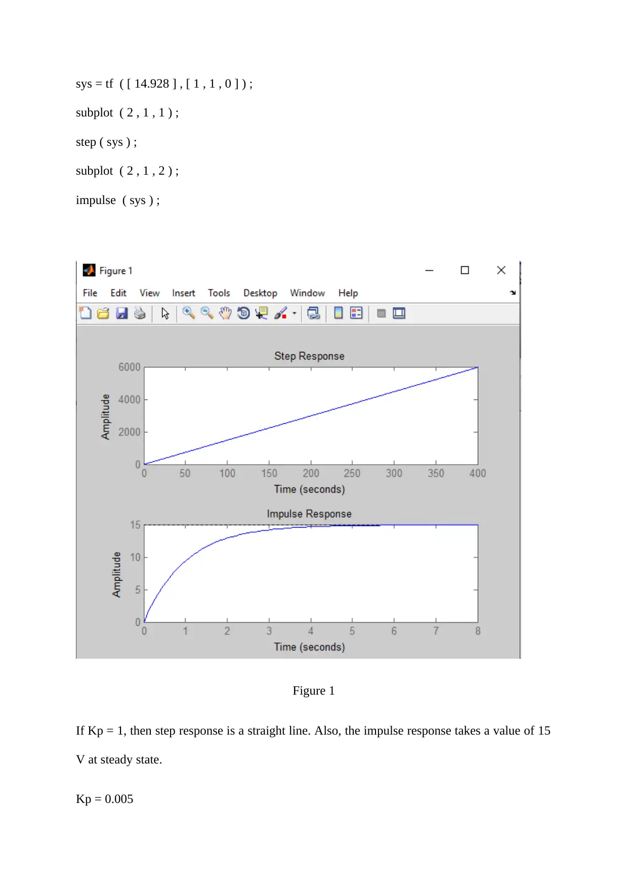
Figure 1
If Kp = 1, then step response is a straight line. Also, the impulse response takes a value of 15
V at steady state.
Kp = 0.005
subplot ( 2 , 1 , 1 ) ;
step ( sys ) ;
subplot ( 2 , 1 , 2 ) ;
impulse ( sys ) ;
Figure 1
If Kp = 1, then step response is a straight line. Also, the impulse response takes a value of 15
V at steady state.
Kp = 0.005
Matlab Code :
sys = tf ( [ 14.928 * 0.005 ] , [ 1 , 1 , 0 ] ) ;
subplot ( 2 , 1 , 1 ) ;
step ( sys ) ;
subplot ( 2 , 1 , 2 ) ;
impulse ( sys ) ;
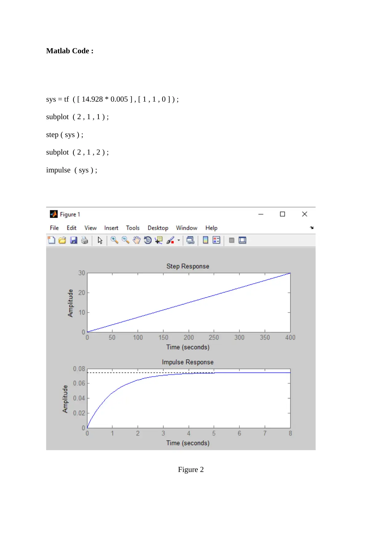
Figure 2
sys = tf ( [ 14.928 * 0.005 ] , [ 1 , 1 , 0 ] ) ;
subplot ( 2 , 1 , 1 ) ;
step ( sys ) ;
subplot ( 2 , 1 , 2 ) ;
impulse ( sys ) ;
Figure 2
If Kp = 0.005, then step response is a straight line. Also, the impulse response takes a value
of 0.075 V at steady state.
Kp = 0.01
Matlab Code :
sys = tf ( [ 14.928 * 0.01 ] , [ 1 , 1 , 0 ] ) ;
subplot ( 2 , 1 , 1 ) ;
step ( sys ) ;
subplot ( 2 , 1 , 2 ) ;
impulse ( sys ) ;
of 0.075 V at steady state.
Kp = 0.01
Matlab Code :
sys = tf ( [ 14.928 * 0.01 ] , [ 1 , 1 , 0 ] ) ;
subplot ( 2 , 1 , 1 ) ;
step ( sys ) ;
subplot ( 2 , 1 , 2 ) ;
impulse ( sys ) ;
Paraphrase This Document
Need a fresh take? Get an instant paraphrase of this document with our AI Paraphraser
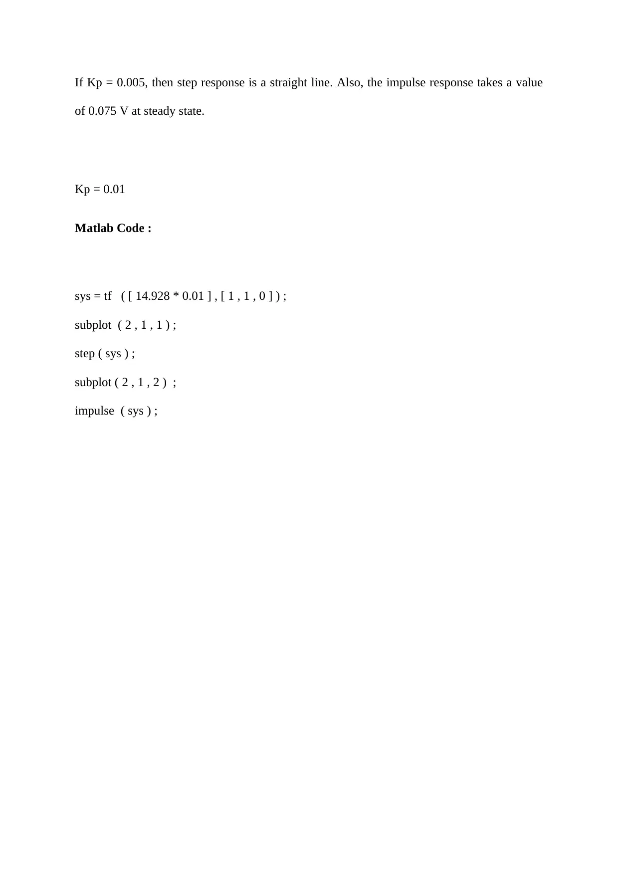
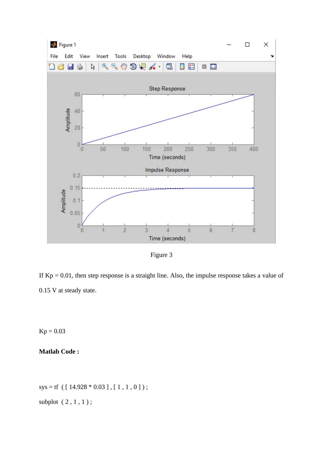
Figure 3
If Kp = 0.01, then step response is a straight line. Also, the impulse response takes a value of
0.15 V at steady state.
Kp = 0.03
Matlab Code :
sys = tf ( [ 14.928 * 0.03 ] , [ 1 , 1 , 0 ] ) ;
subplot ( 2 , 1 , 1 ) ;
If Kp = 0.01, then step response is a straight line. Also, the impulse response takes a value of
0.15 V at steady state.
Kp = 0.03
Matlab Code :
sys = tf ( [ 14.928 * 0.03 ] , [ 1 , 1 , 0 ] ) ;
subplot ( 2 , 1 , 1 ) ;
step ( sys ) ;
subplot ( 2 , 1 , 2 ) ;
impulse ( sys ) ;
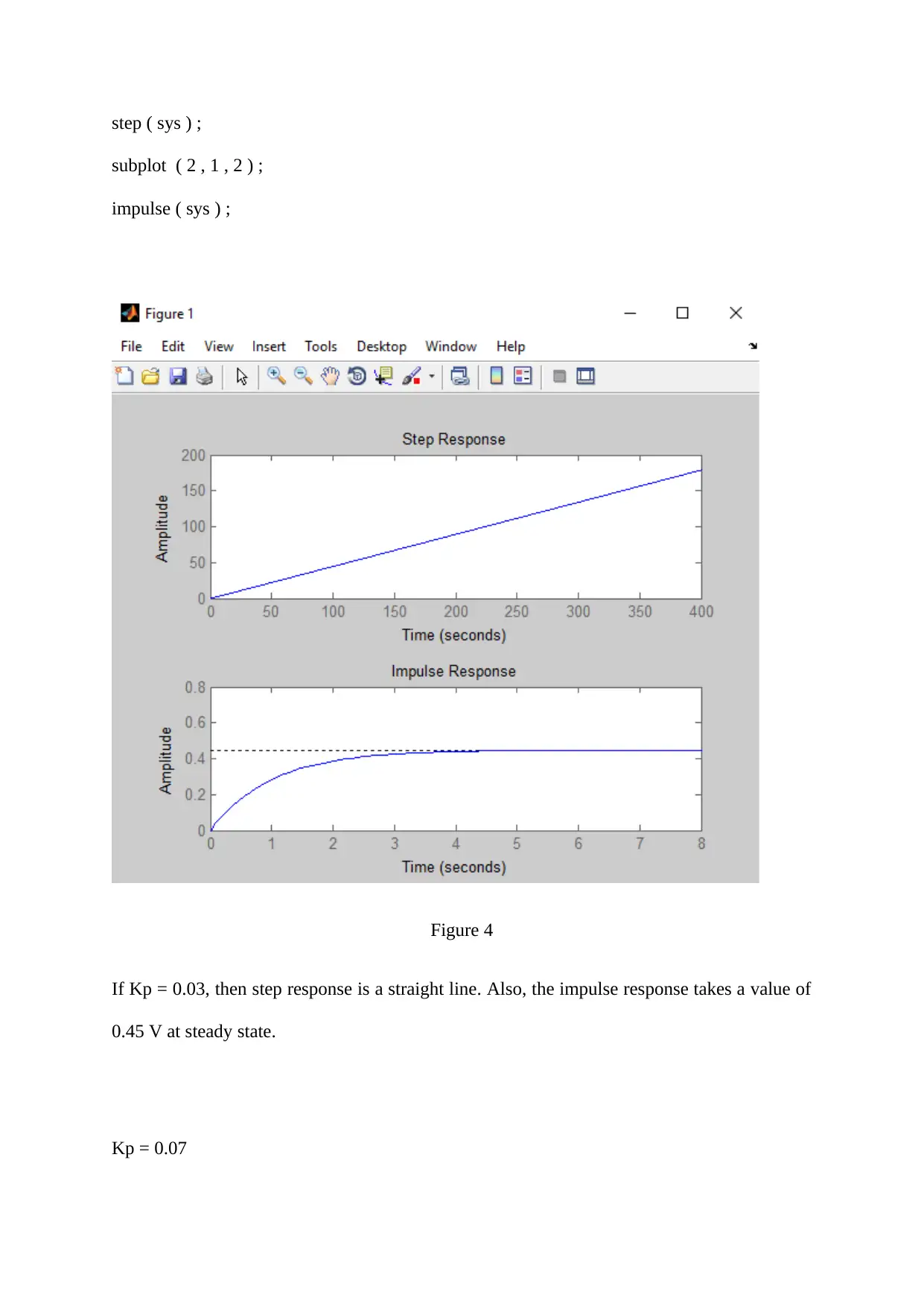
Figure 4
If Kp = 0.03, then step response is a straight line. Also, the impulse response takes a value of
0.45 V at steady state.
Kp = 0.07
subplot ( 2 , 1 , 2 ) ;
impulse ( sys ) ;
Figure 4
If Kp = 0.03, then step response is a straight line. Also, the impulse response takes a value of
0.45 V at steady state.
Kp = 0.07
Matlab Code :
sys = tf ( [ 14.928 * 0.07 ] , [ 1 , 1 , 0 ] ) ;
subplot ( 2 , 1 , 1 ) ;
step ( sys ) ;
subplot ( 2 , 1 , 2 ) ;
impulse ( sys ) ;
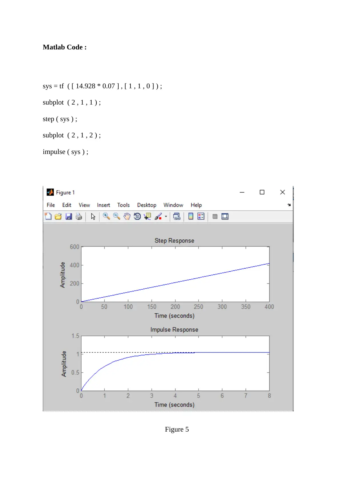
Figure 5
sys = tf ( [ 14.928 * 0.07 ] , [ 1 , 1 , 0 ] ) ;
subplot ( 2 , 1 , 1 ) ;
step ( sys ) ;
subplot ( 2 , 1 , 2 ) ;
impulse ( sys ) ;
Figure 5
Secure Best Marks with AI Grader
Need help grading? Try our AI Grader for instant feedback on your assignments.
If Kp = 0.07, then step response is a straight line. Also, the impulse response takes a value of
1.1 V at steady state.
PD Controller
The MATLAB plot command is used here.
Evaluation of parameters ( of the transient responses )
The effect of gain, Kp on the parameters
Transient Responses Plots for different values of Kd ( PD Controller ) for 1 co – ordinate
system :
The MATLAB plot command is used here.
Kd = 0.002
Matlab Code :
sys = tf ( [ 14.928 * 0.002 , 14.928 * 0.02 ] , [ 1 , 1 , 0 ] ) ;
subplot ( 2 , 1 , 1 ) ;
step ( sys ) ;
subplot ( 2 , 1 , 2 ) ;
impulse ( sys ) ;
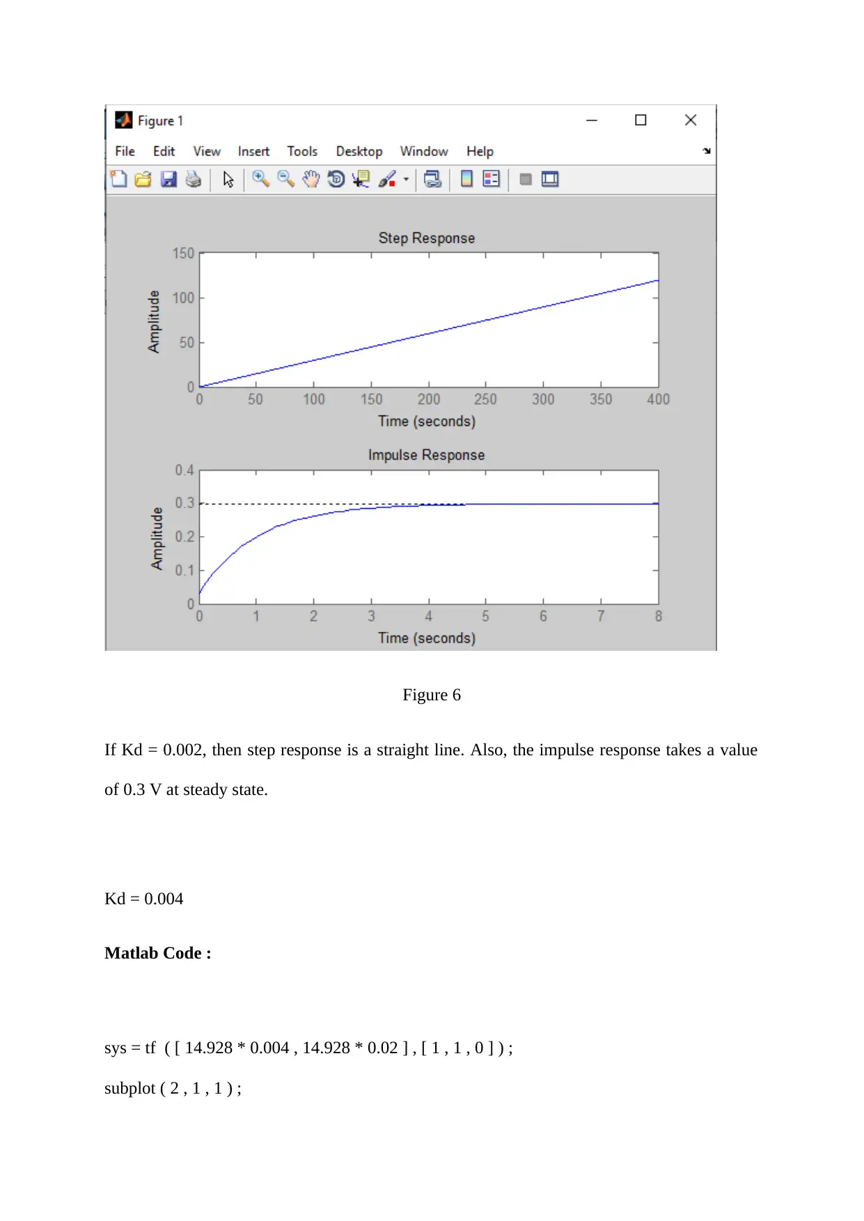
Figure 6
If Kd = 0.002, then step response is a straight line. Also, the impulse response takes a value
of 0.3 V at steady state.
Kd = 0.004
Matlab Code :
sys = tf ( [ 14.928 * 0.004 , 14.928 * 0.02 ] , [ 1 , 1 , 0 ] ) ;
subplot ( 2 , 1 , 1 ) ;
If Kd = 0.002, then step response is a straight line. Also, the impulse response takes a value
of 0.3 V at steady state.
Kd = 0.004
Matlab Code :
sys = tf ( [ 14.928 * 0.004 , 14.928 * 0.02 ] , [ 1 , 1 , 0 ] ) ;
subplot ( 2 , 1 , 1 ) ;
step ( sys ) ;
subplot ( 2 , 1 , 2 ) ;
impulse ( sys ) ;
Figure 7
If Kd = 0.004, then step response is a straight line. Also, the impulse response takes a value
of 0.3 V at steady state.
Kd = 0.006
subplot ( 2 , 1 , 2 ) ;
impulse ( sys ) ;
Figure 7
If Kd = 0.004, then step response is a straight line. Also, the impulse response takes a value
of 0.3 V at steady state.
Kd = 0.006
Paraphrase This Document
Need a fresh take? Get an instant paraphrase of this document with our AI Paraphraser
Matlab Code :
sys = tf ( [ 14.928 * 0.006 , 14.928 * 0.02 ] , [ 1 , 1 , 0 ] ) ;
subplot ( 2 , 1 , 1 ) ;
step ( sys ) ;
subplot ( 2 , 1 , 2 ) ;
impulse ( sys ) ;
Figure 8
sys = tf ( [ 14.928 * 0.006 , 14.928 * 0.02 ] , [ 1 , 1 , 0 ] ) ;
subplot ( 2 , 1 , 1 ) ;
step ( sys ) ;
subplot ( 2 , 1 , 2 ) ;
impulse ( sys ) ;
Figure 8
If Kd = 0.006, then step response is a straight line. Also, the impulse response takes a value
of 0.3 V at steady state.
Speed Control
Transient Responses Plots for different values of Kp ( on speed ) for 1 co – ordinate
system :
The MATLAB plot command is used here.
Derivation of closed loop system transfer function for controller :
The open loop transfer function is :
X ( s ) / Y ( s ) = khw x 1/ s ( J s + C )
= 14.928 / s ( J s + C )
If PD controller is added ,
Open loop transfer function = 14.928 ( Kp + s Kd ) / s ( J s + C )
Closed loop transfer function = 1 + 14.928 ( Kp + s Kd ) / s ( J s + C )
= [ s ( J s + C ) + 14.928 ( Kp + s Kd ) ] / s ( J s + C )
Effect of change of gains Kp and Kd on the location of poles :
If Kd = 0.002 , kp = 0.02:
Matlab Code :
s = tf ( ' s ' ) ;
G = ( 0.02 + ( 0.002 * s ) ) / ( s ^ 2 + s ) ;
k = 14.928 ;
T = feedback ( G * k , 1 ) ;
pzmap ( T ) ;
grid
If Kd = 0.002 , kp = 0.02:
Matlab Code :
s = tf ( ' s ' ) ;
G = ( 0.02 + ( 0.002 * s ) ) / ( s ^ 2 + s ) ;
k = 14.928 ;
T = feedback ( G * k , 1 ) ;
pzmap ( T ) ;
grid
Secure Best Marks with AI Grader
Need help grading? Try our AI Grader for instant feedback on your assignments.
Figure 9
If Kd = 0.002 , kp = 0.02, then 1 zero is located on real axis and 2 imaginary poles are
located in LHS side.
If Kd = 0.004, kp = 0.02 :
The MATLAB code is written by taking the open loop transfer function as per the parameters
provided and then adding unity feedback to obtain the closed loop transfer function . This
function’s response is then evaluated.
Matlab Code :
s = tf ( ' s ' ) ;
G = ( 0.02 + ( 0.004 * s ) ) / ( s ^ 2 + s ) ;
k = 14.928 ;
T = feedback ( G * k , 1 ) ;
pzmap ( T ) ;
grid
G = ( 0.02 + ( 0.004 * s ) ) / ( s ^ 2 + s ) ;
k = 14.928 ;
T = feedback ( G * k , 1 ) ;
pzmap ( T ) ;
grid
Figure 10
If Kd = 0.004 , kp = 0.02, then 1 zero is located on real axis but now its near to origin as
compared to previous case and 2 imaginary poles are located in LHS side.
Effect of increase in Kp (proportional gain) in servo system for speed control on the response
of the closed loop system.
Kd = 0.006 , kp = 0.02
Matlab Code :
s = tf ( ' s ' ) ;
G = ( 0.02 + ( 0.006 * s ) ) / ( s ^ 2 + s ) ;
k = 14.928 ;
T = feedback ( G * k , 1 ) ;
pzmap ( T ) ;
grid
Paraphrase This Document
Need a fresh take? Get an instant paraphrase of this document with our AI Paraphraser
Figure 11
If Kd = 0.006 , kp = 0.02, then 1 zero is located on real axis but now its near to origin as
compared to previous case and 2 imaginary poles are located in LHS side.
Kd = 0.004 , kp = 0.01
Matlab Code :
s = tf ( ' s ' ) ;
G = ( 0.01 + ( 0 .004 * s ) ) / ( s ^ 2 + s ) ;
If Kd = 0.006 , kp = 0.02, then 1 zero is located on real axis but now its near to origin as
compared to previous case and 2 imaginary poles are located in LHS side.
Kd = 0.004 , kp = 0.01
Matlab Code :
s = tf ( ' s ' ) ;
G = ( 0.01 + ( 0 .004 * s ) ) / ( s ^ 2 + s ) ;
k = 14.928 ;
T = feedback ( G * k , 1 ) ;
pzmap ( T ) ;
grid
Figure 12
If Kd = 0.004 , kp = 0.01, then 1 zero is located on real axis but now its near to origin as
compared to previous case and 2 poles are located in LHS side on the real axis.
T = feedback ( G * k , 1 ) ;
pzmap ( T ) ;
grid
Figure 12
If Kd = 0.004 , kp = 0.01, then 1 zero is located on real axis but now its near to origin as
compared to previous case and 2 poles are located in LHS side on the real axis.
Kd = 0.004 , kp = 0.008
Matlab Code :
s = tf ( ' s ' ) ;
G = ( 0.008 + ( 0.004 * s ) ) / ( s ^ 2 + s ) ;
k = 14.928 ;
T = feedback ( G * k , 1 ) ;
pzmap ( T ) ;
grid
Matlab Code :
s = tf ( ' s ' ) ;
G = ( 0.008 + ( 0.004 * s ) ) / ( s ^ 2 + s ) ;
k = 14.928 ;
T = feedback ( G * k , 1 ) ;
pzmap ( T ) ;
grid
Secure Best Marks with AI Grader
Need help grading? Try our AI Grader for instant feedback on your assignments.
Figure 13
If Kd = 0.004 , kp = 0.008, then 1 zero is located on real axis but now its near to origin as
compared to previous case and 2 poles are located in LHS side on the real axis near to the
origin.
Conclusion :
Hence, the control system under consideration has been studied in detail. The various
parameters have been changed and the response has been studied for all the cases. Every case
is run on the MATLAB software to observe the step response and the impulse response.
These systems are then compared in terms of various parameters. This gives an insight into
how the response is affected on changing the parameter values. Also, the location of poles
and zeros is studied for the closed loop system when various parameter values are changed.
References
[1] Goman, M. , “Dynamics and Control of Mechanical Systems” – lecture in Dynamics
notes on DMU Black Board, 2015.
[2] Ulanicki, B., “Dynamics & Control of Mechani cal Systems” – lecture in Dynamics notes
on DMU Black Board, 2018.
[3] Guerrero, Daniel Palomo, and Francisco J. Jiménez-Espadafor. "Torsional system
dynamics of low speed diesel engines based on instantaneous torque: Application to engine
diagnosis." Mechanical Systems and Signal Processing 116 (2019):
1 out of 24
Related Documents
Your All-in-One AI-Powered Toolkit for Academic Success.
+13062052269
info@desklib.com
Available 24*7 on WhatsApp / Email
Unlock your academic potential
© 2024 | Zucol Services PVT LTD | All rights reserved.