ENV3105 Hydrology S2 2019

Evaluation of Modules 2 to 5's chosen learning goals in ENV3105 Hydrology S2 2019. Measurement and presentation of rainfall and streamflow data, analysis of flood frequency and estimation of flood design, design IFD rainfall, and estimation of peak discharges.

Running head: ENV3105 HYDROLOGY S2 2019 1
ENV3105 Hydrology S2 2019
Firstname Lastname
Name of Institution

ENV3105 HYDROLOGY S2 2019 2
Project Background
This evaluation is intended to evaluate your accomplishment of Modules 2 to 5's chosen learning
goals. The assignment includes (a) measurement and presentation of rainfall and streamflow
data, (b) analysis of flood frequency and estimation of flood design, (c) design IFD rainfall, and
(d) estimation of peak discharges. Historical streamflow and rainfall information will work with
you. The purpose of the task is to strengthen and extend your understanding of hydrological
techniques and the (significant) uncertainty connected with the assessment of design floods.
To show how hydrology can be integrated into engineering practice, a hypothetical project has
been designed. Although the project is imaginary (and unlikely to receive permission to
proceed), the different hydrological tasks included in the project are representative of what you
may encounter after graduating.
The aim of the task is to predict the design flood discharges for the stream gage site (142001A
Caboolture River at Upper Caboolture under the Pine Basin) for a range of annual excess
probabilities (2, 10 and 100-year ARIs corresponding to 50%, 10% and 1% AEPs respectively).
The assessment of flood frequency (FFA) will be based on the results of four methods: the
Annual Series, the Partial Series, the Palmen & Weeks process (Palmen and Weeks, 2014) and
the fresh Regional Flood Frequency Estimate (RFFE) instrument established as part of the
AR&R update (Rahman et al, 2015).
The task is based on the following key responsibilities:
1. Obtaining and reviewing information from streamflow
2. Annual FFA series based on fitting a distribution of the Pearson 3 log (LP3) to the maximum
annual flow
3. Partial FFA series based on a maximum of monthly release.
4. Design estimation of release using the techniques Palmen & Weeks (2014) and RFFE.
5. Compilation of estimates and choice of a set of discharges from the design flood, based on the
above inputs

ENV3105 HYDROLOGY S2 2019 3
6. Evaluation of the rainfall frequency connected with flood event in January 2011.
7. Preparing a report on the task
3.1 Streamflow data
Basic stream gauge Data
Information Required Answer
Basin name Pine Basin
Creek name Caboolture River at Upper Caboolture
Location of site Caboolture, 27o05’52.1”S (latitude) and
152o53’26.2”E (longitude)
Catchment area 94 km2 (9400 hectares)
Streamgauging commencement data 01/10/1965
Rainfall (data source A and AT) data
measurement start date
17/09/1990
Rainfall data resolution Daily
Maximum instantaneous discharge (in
cumecs) value and occurrence data (from data
source A)
604.482 cumecs, 11/01/2011
2526.620 cumecs, 15/03/2019
HYDRAULIC CONTROL AND RATING CURVE
Information Required Answer
Type of control Sand gravel

ENV3105 HYDROLOGY S2 2019 4
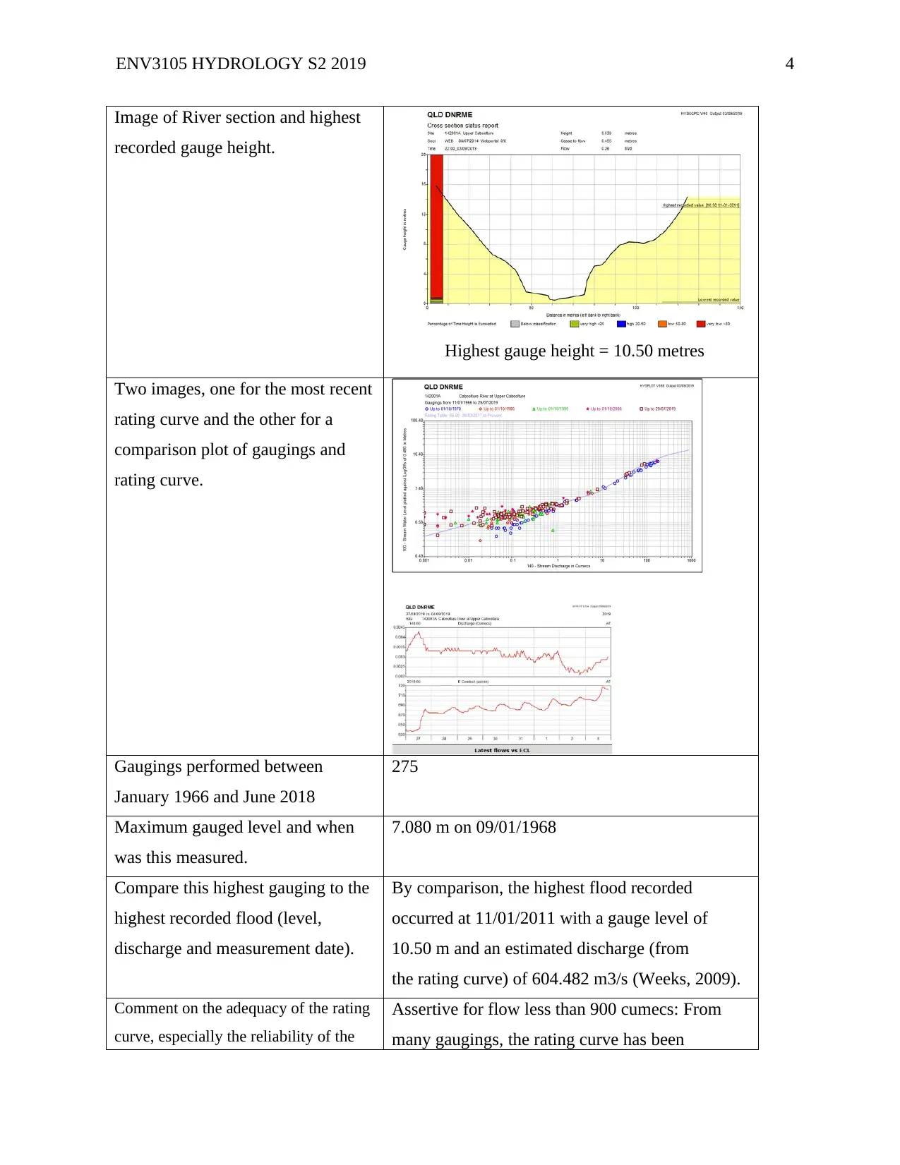
Image of River section and highest
recorded gauge height.
Highest gauge height = 10.50 metres
Two images, one for the most recent
rating curve and the other for a
comparison plot of gaugings and
rating curve.
Gaugings performed between
January 1966 and June 2018
275
Maximum gauged level and when
was this measured.
7.080 m on 09/01/1968
Compare this highest gauging to the
highest recorded flood (level,
discharge and measurement date).
By comparison, the highest flood recorded
occurred at 11/01/2011 with a gauge level of
10.50 m and an estimated discharge (from
the rating curve) of 604.482 m3/s (Weeks, 2009).
Comment on the adequacy of the rating
curve, especially the reliability of the
Assertive for flow less than 900 cumecs: From
many gaugings, the rating curve has been

ENV3105 HYDROLOGY S2 2019 5
discharges associated with different
flood levels.
confirmed for flows (<900 m3/s (Rahman, 2008).
This offers self-assurance in discharges in this
flow range only.
Low accuracy for flows more than 900 cumecs:
The largest observed flood discharge is
approximately 2526.620 m3/s. Flood discharges
are based on a theoretical rating curve and is
expected that the accuracy is low to moderate.
FLOW DURATION CURVE
Information Required Answer
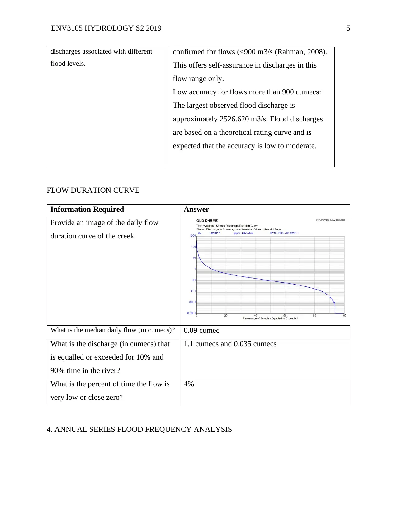
Provide an image of the daily flow
duration curve of the creek.
What is the median daily flow (in cumecs)? 0.09 cumec
What is the discharge (in cumecs) that
is equalled or exceeded for 10% and
90% time in the river?
1.1 cumecs and 0.035 cumecs
What is the percent of time the flow is
very low or close zero?
4%
4. ANNUAL SERIES FLOOD FREQUENCY ANALYSIS

ENV3105 HYDROLOGY S2 2019 6
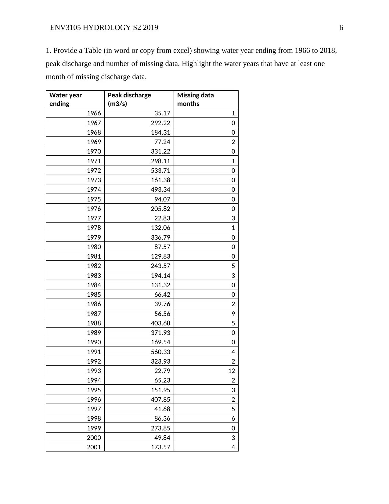
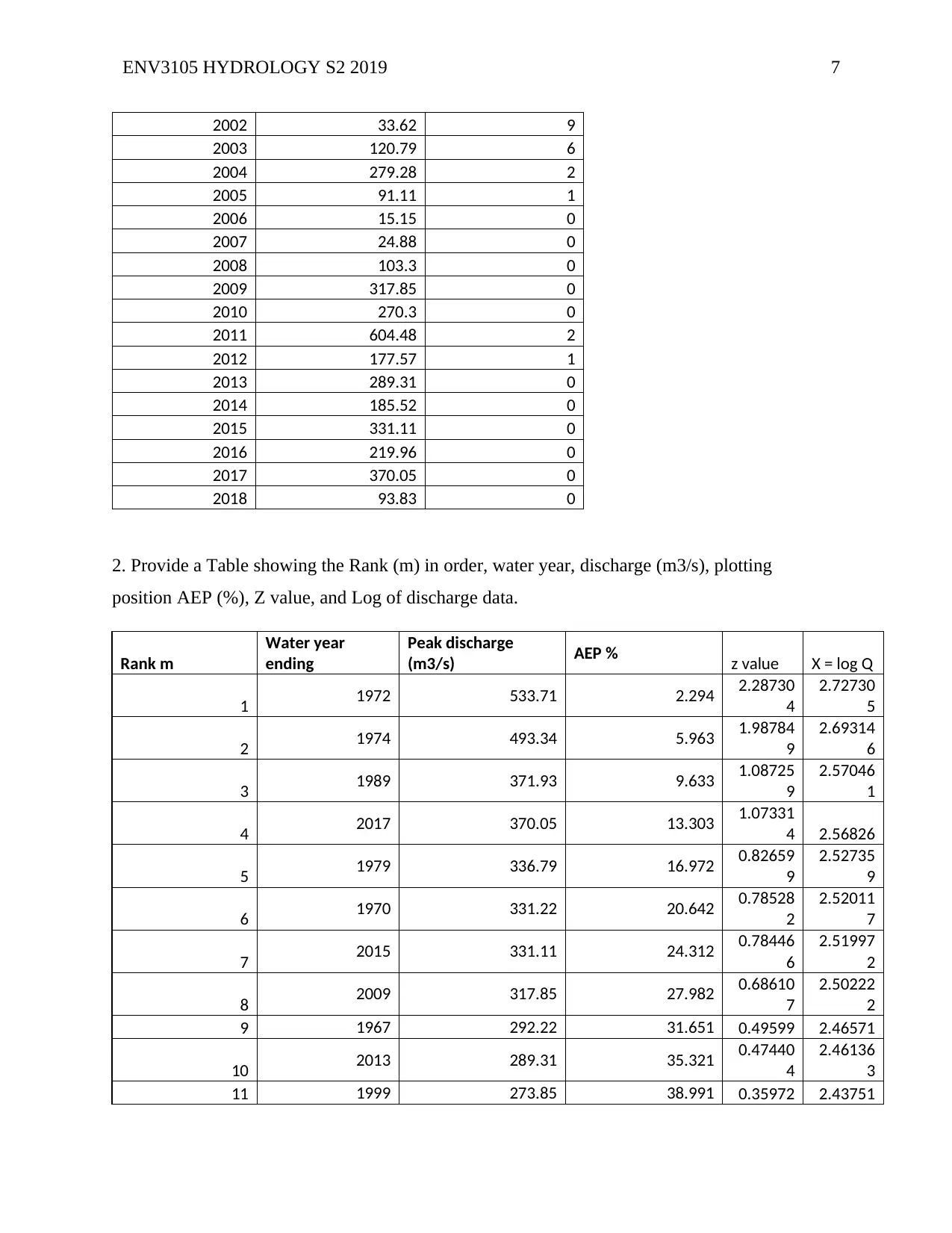
1. Provide a Table (in word or copy from excel) showing water year ending from 1966 to 2018,
peak discharge and number of missing data. Highlight the water years that have at least one
month of missing discharge data.
Water year
ending
Peak discharge
(m3/s)
Missing data
months
1966 35.17 1
1967 292.22 0
1968 184.31 0
1969 77.24 2
1970 331.22 0
1971 298.11 1
1972 533.71 0
1973 161.38 0
1974 493.34 0
1975 94.07 0
1976 205.82 0
1977 22.83 3
1978 132.06 1
1979 336.79 0
1980 87.57 0
1981 129.83 0
1982 243.57 5
1983 194.14 3
1984 131.32 0
1985 66.42 0
1986 39.76 2
1987 56.56 9
1988 403.68 5
1989 371.93 0
1990 169.54 0
1991 560.33 4
1992 323.93 2
1993 22.79 12
1994 65.23 2
1995 151.95 3
1996 407.85 2
1997 41.68 5
1998 86.36 6
1999 273.85 0
2000 49.84 3
2001 173.57 4

ENV3105 HYDROLOGY S2 2019 7
2002 33.62 9
2003 120.79 6
2004 279.28 2
2005 91.11 1
2006 15.15 0
2007 24.88 0
2008 103.3 0
2009 317.85 0
2010 270.3 0
2011 604.48 2
2012 177.57 1
2013 289.31 0
2014 185.52 0
2015 331.11 0
2016 219.96 0
2017 370.05 0
2018 93.83 0
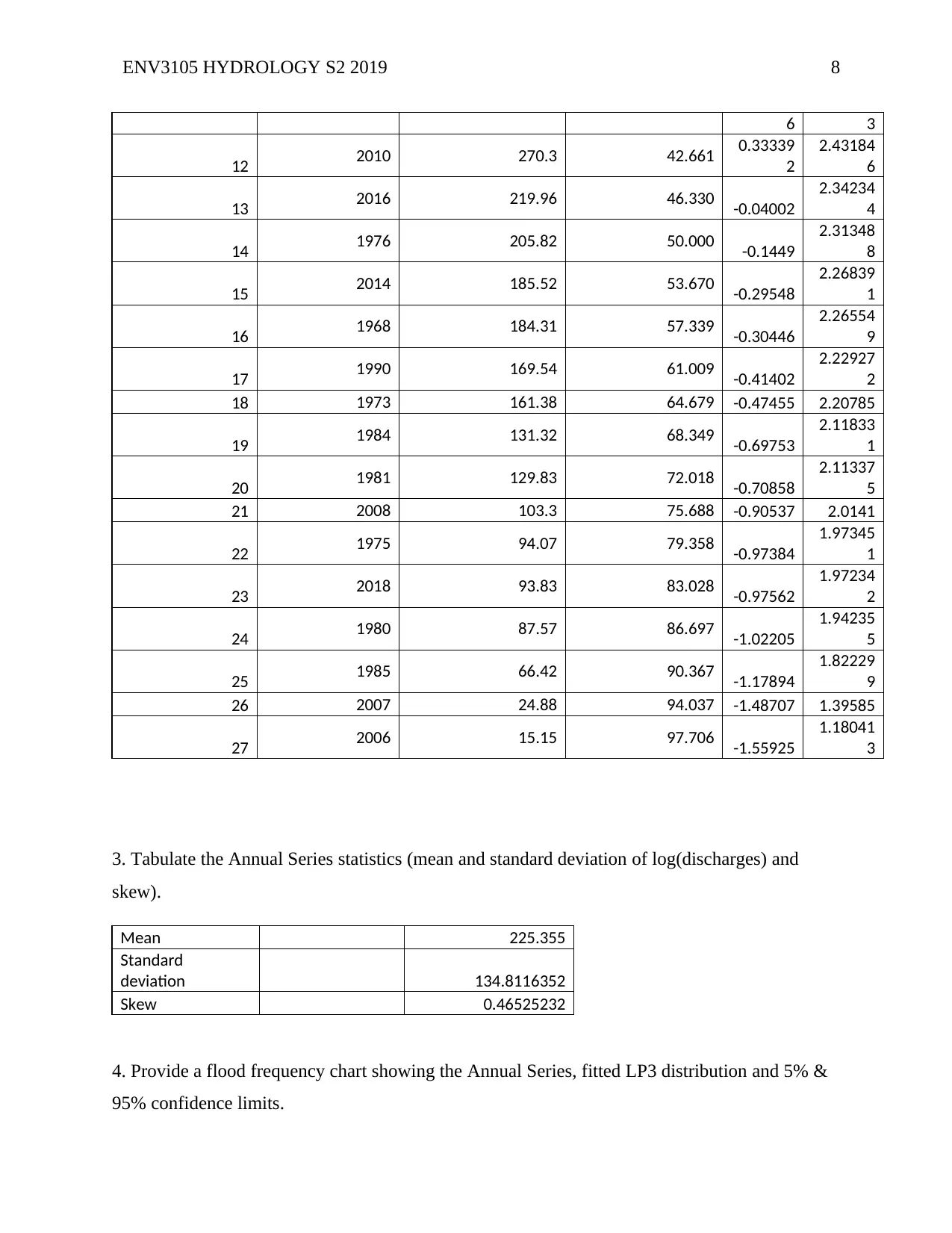
2. Provide a Table showing the Rank (m) in order, water year, discharge (m3/s), plotting
position AEP (%), Z value, and Log of discharge data.
Rank m
Water year
ending
Peak discharge
(m3/s) AEP % z value X = log Q
1 1972 533.71 2.294 2.28730
4
2.72730
5
2 1974 493.34 5.963 1.98784
9
2.69314
6
3 1989 371.93 9.633 1.08725
9
2.57046
1
4 2017 370.05 13.303 1.07331
4 2.56826
5 1979 336.79 16.972 0.82659
9
2.52735
9
6 1970 331.22 20.642 0.78528
2
2.52011
7
7 2015 331.11 24.312 0.78446
6
2.51997
2
8 2009 317.85 27.982 0.68610
7
2.50222
2
9 1967 292.22 31.651 0.49599 2.46571
10 2013 289.31 35.321 0.47440
4
2.46136
3
11 1999 273.85 38.991 0.35972 2.43751

ENV3105 HYDROLOGY S2 2019 8
6 3
12 2010 270.3 42.661 0.33339
2
2.43184
6
13 2016 219.96 46.330 -0.04002
2.34234
4
14 1976 205.82 50.000 -0.1449
2.31348
8
15 2014 185.52 53.670 -0.29548
2.26839
1
16 1968 184.31 57.339 -0.30446
2.26554
9
17 1990 169.54 61.009 -0.41402
2.22927
2
18 1973 161.38 64.679 -0.47455 2.20785
19 1984 131.32 68.349 -0.69753
2.11833
1
20 1981 129.83 72.018 -0.70858
2.11337
5
21 2008 103.3 75.688 -0.90537 2.0141
22 1975 94.07 79.358 -0.97384
1.97345
1
23 2018 93.83 83.028 -0.97562
1.97234
2
24 1980 87.57 86.697 -1.02205
1.94235
5
25 1985 66.42 90.367 -1.17894
1.82229
9
26 2007 24.88 94.037 -1.48707 1.39585
27 2006 15.15 97.706 -1.55925
1.18041
3
3. Tabulate the Annual Series statistics (mean and standard deviation of log(discharges) and
skew).
Mean 225.355
Standard
deviation 134.8116352
Skew 0.46525232
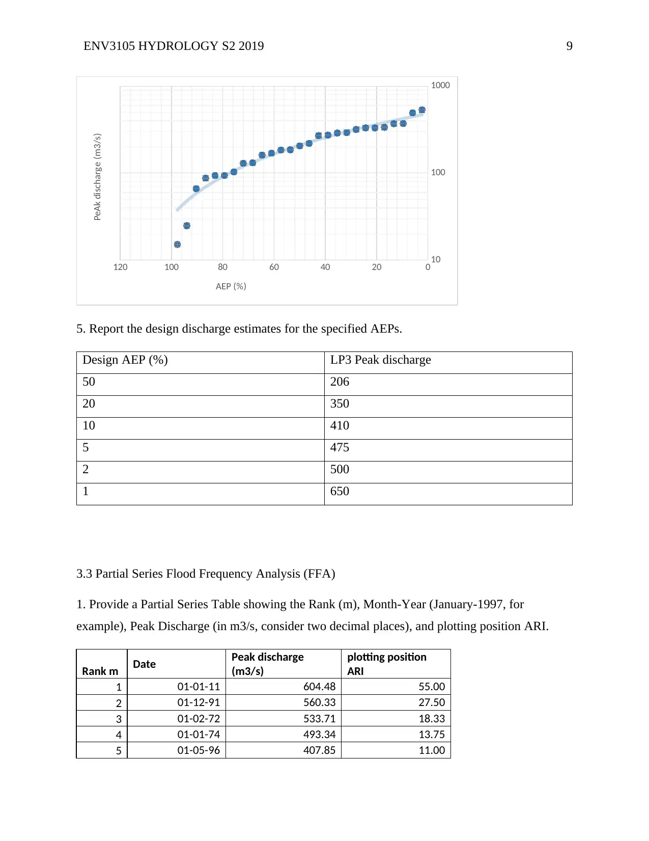
4. Provide a flood frequency chart showing the Annual Series, fitted LP3 distribution and 5% &
95% confidence limits.

ENV3105 HYDROLOGY S2 2019 9
020406080100120 10
100
1000
AEP (%)
PeAk discharge (m3/s)
5. Report the design discharge estimates for the specified AEPs.
Design AEP (%) LP3 Peak discharge
50 206
20 350
10 410
5 475
2 500
1 650
3.3 Partial Series Flood Frequency Analysis (FFA)
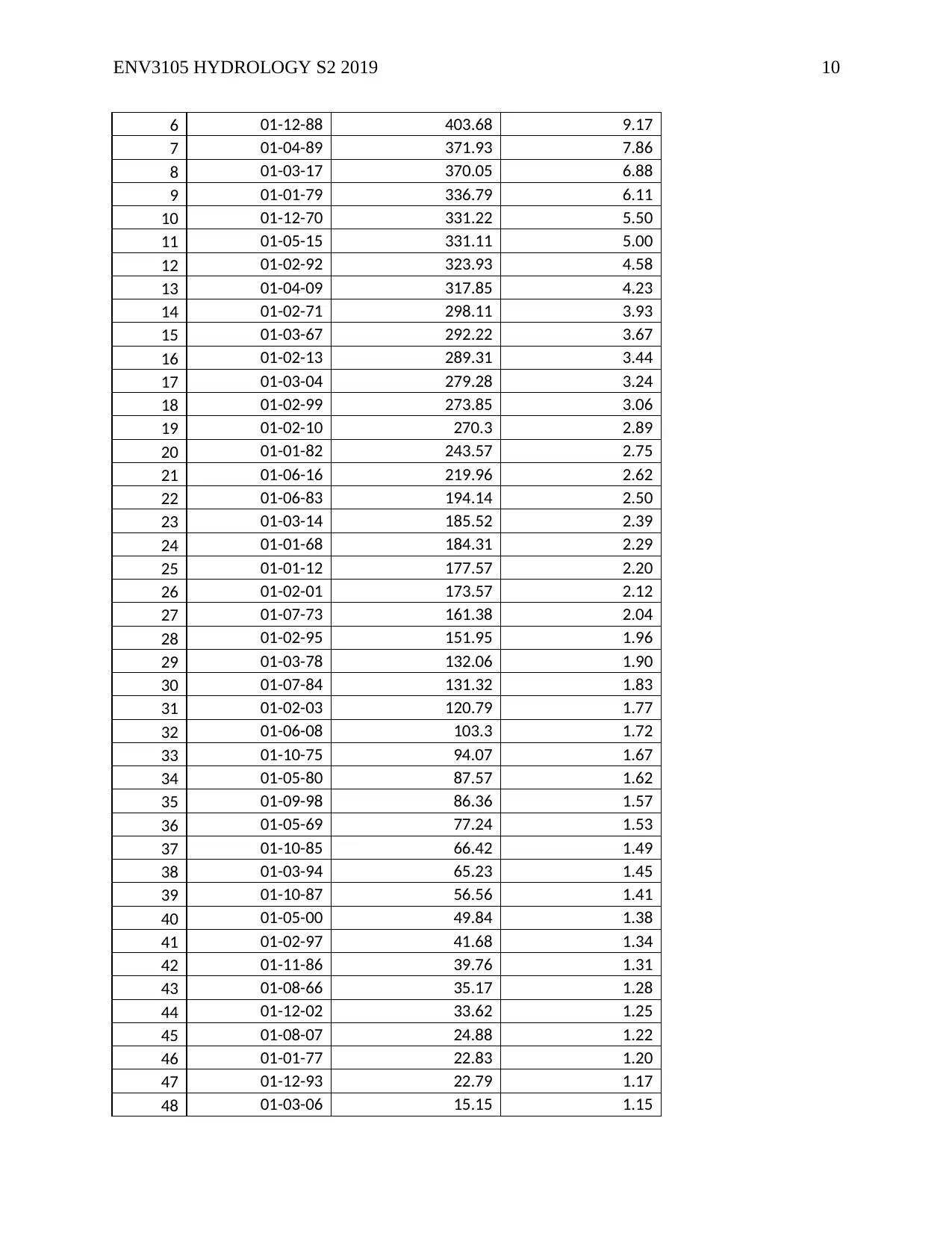
1. Provide a Partial Series Table showing the Rank (m), Month-Year (January-1997, for
example), Peak Discharge (in m3/s, consider two decimal places), and plotting position ARI.
Rank m Date Peak discharge
(m3/s)
plotting position
ARI
1 01-01-11 604.48 55.00
2 01-12-91 560.33 27.50
3 01-02-72 533.71 18.33
4 01-01-74 493.34 13.75
5 01-05-96 407.85 11.00

ENV3105 HYDROLOGY S2 2019 10
6 01-12-88 403.68 9.17
7 01-04-89 371.93 7.86
8 01-03-17 370.05 6.88
9 01-01-79 336.79 6.11
10 01-12-70 331.22 5.50
11 01-05-15 331.11 5.00
12 01-02-92 323.93 4.58
13 01-04-09 317.85 4.23
14 01-02-71 298.11 3.93
15 01-03-67 292.22 3.67
16 01-02-13 289.31 3.44
17 01-03-04 279.28 3.24
18 01-02-99 273.85 3.06
19 01-02-10 270.3 2.89
20 01-01-82 243.57 2.75
21 01-06-16 219.96 2.62
22 01-06-83 194.14 2.50
23 01-03-14 185.52 2.39
24 01-01-68 184.31 2.29
25 01-01-12 177.57 2.20
26 01-02-01 173.57 2.12
27 01-07-73 161.38 2.04
28 01-02-95 151.95 1.96
29 01-03-78 132.06 1.90
30 01-07-84 131.32 1.83
31 01-02-03 120.79 1.77
32 01-06-08 103.3 1.72
33 01-10-75 94.07 1.67
34 01-05-80 87.57 1.62
35 01-09-98 86.36 1.57
36 01-05-69 77.24 1.53
37 01-10-85 66.42 1.49
38 01-03-94 65.23 1.45
39 01-10-87 56.56 1.41
40 01-05-00 49.84 1.38
41 01-02-97 41.68 1.34
42 01-11-86 39.76 1.31
43 01-08-66 35.17 1.28
44 01-12-02 33.62 1.25
45 01-08-07 24.88 1.22
46 01-01-77 22.83 1.20
47 01-12-93 22.79 1.17
48 01-03-06 15.15 1.15

ENV3105 HYDROLOGY S2 2019 11
N = 48 years because no month with no data is included.
K = N = 48. This corresponds to floods that exceed 15.15 m3/s (Weinman, n.d.).
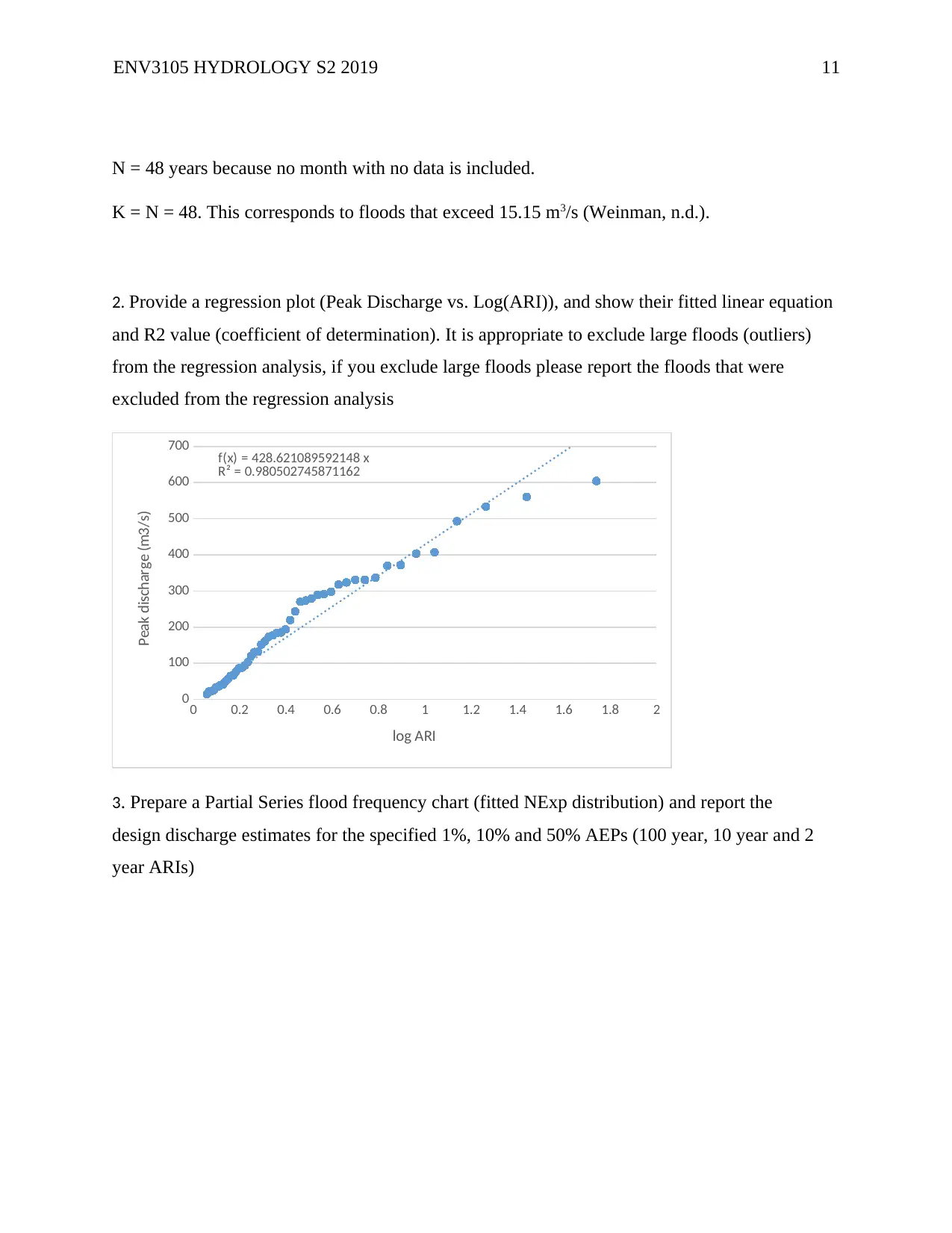
2. Provide a regression plot (Peak Discharge vs. Log(ARI)), and show their fitted linear equation
and R2 value (coefficient of determination). It is appropriate to exclude large floods (outliers)
from the regression analysis, if you exclude large floods please report the floods that were
excluded from the regression analysis
0 0.2 0.4 0.6 0.8 1 1.2 1.4 1.6 1.8 2
0
100
200
300
400
500
600
700 f(x) = 428.621089592148 x
R² = 0.980502745871162
log ARI
Peak discharge (m3/s)
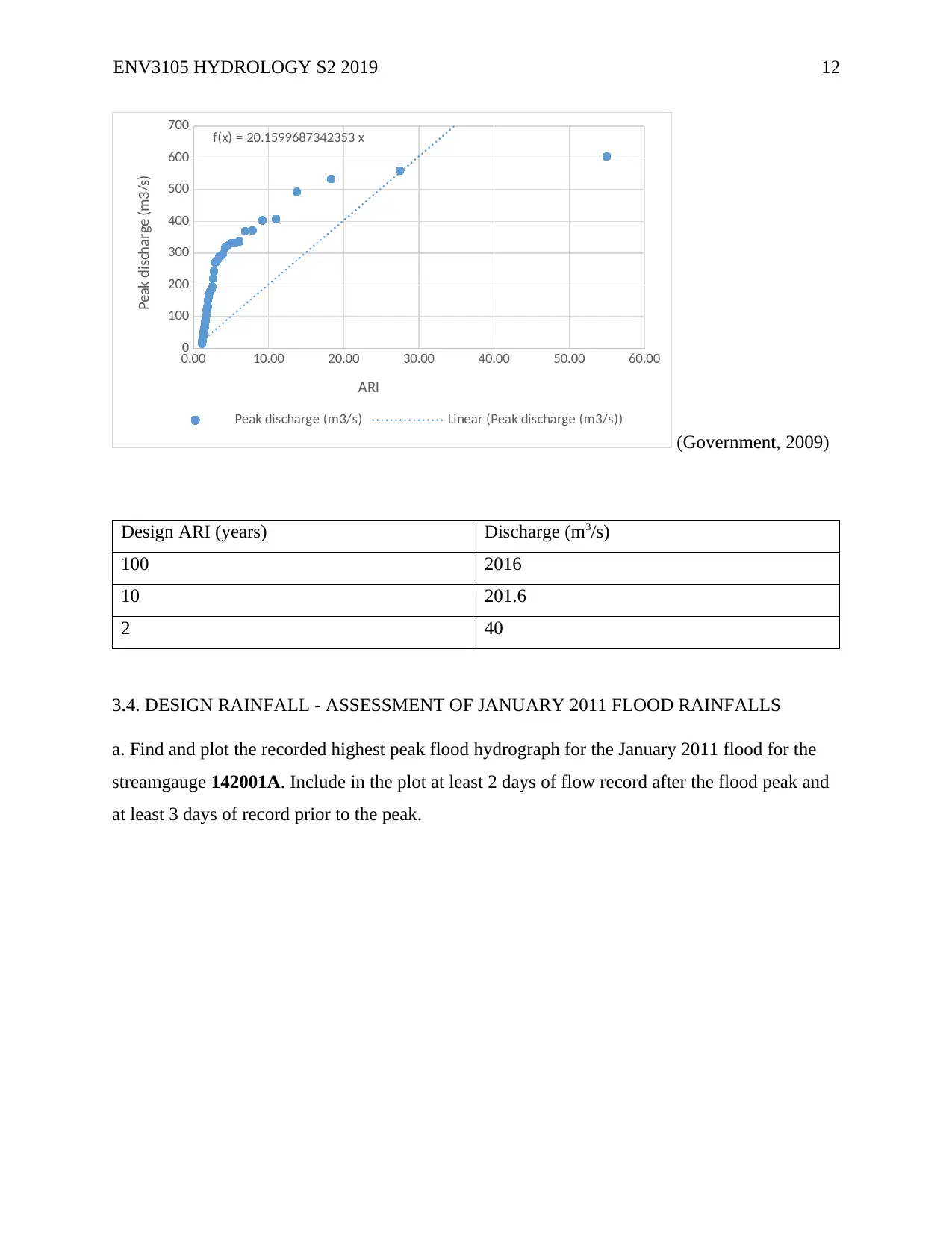
3. Prepare a Partial Series flood frequency chart (fitted NExp distribution) and report the
design discharge estimates for the specified 1%, 10% and 50% AEPs (100 year, 10 year and 2
year ARIs)

ENV3105 HYDROLOGY S2 2019 12
0.00 10.00 20.00 30.00 40.00 50.00 60.00
0
100
200
300
400
500
600
700 f(x) = 20.1599687342353 x
Peak discharge (m3/s) Linear (Peak discharge (m3/s))
ARI
Peak discharge (m3/s)
(Government, 2009)
Design ARI (years) Discharge (m3/s)
100 2016
10 201.6
2 40
3.4. DESIGN RAINFALL - ASSESSMENT OF JANUARY 2011 FLOOD RAINFALLS
a. Find and plot the recorded highest peak flood hydrograph for the January 2011 flood for the
streamgauge 142001A. Include in the plot at least 2 days of flow record after the flood peak and
at least 3 days of record prior to the peak.

ENV3105 HYDROLOGY S2 2019 13
b. Provide the following information from the above-mentioned plot of rainfall and flood
hydrograph for January 2011.
Date and amount of maximum discharge
occurred.
11th January 2011, 70 cumecs
Date and amount of maximum rainfall (mm/day)
occurred.
10th January 2011, 310 mm/day
c. From the plots, you will be able to identify the period of rainfall that was associated with the
flood. Download the hourly rainfalls for this period of time and report the maximum hourly
rainfall depth (in mm) and intensity (in mm/hour) and when (date and time) it was
happened
Time/date: 11:00:00 10th January 2011 55 mm
Rainfall intensity 55 mm/hour
d.

ENV3105 HYDROLOGY S2 2019 14
e.
Annual Exceedance Probability
Duration 50% 10% 1%
1 26 43.5 70.7
1.8 21.28 18.72 15.36
2 20.1 34.4 57.4
3.5 Design Discharge Estimation – Quantile Regression (Palmen and Weeks, 2011) and Regional
Flood Frequency Estimation (RFFE) Methods

ENV3105 HYDROLOGY S2 2019 15
a)
Information Required Answer
Minimum stream gauge record length adopted
in their study.
10 years
Catchment parameters dropped from the list. 1. Stream density
2. 2. Forest area
3. 3. Quaternary sediment area
Significant catchment parameters used in the
QRT based peak discharge estimation
equations
1. Catchment area (km2)
2. 72-hour duration 50 year ARI rainfall
intensity (mm/h)
Probability distribution used in FFA and
parameter estimation technique.
LP3 and Method of Moments.
Probability distribution nd parameter
estimation technique recommended in ARR
2016.
GEV and L-moments
b)

ENV3105 HYDROLOGY S2 2019 16
c)
Streamgauge location -270 latitude, 1530 longitude
Catchment centroid location -27.1050 latitude, 153.0030 longitude
Catchment area (km2) 94
72 hour 50 year rainfall intensity (mm/hr) 7.15
(Weeks, 2011)
d)
ARI Discharge (m3/s)
2 289
5 660
10 787
20 1190
50 1603
100 1883
e.
AEP Discharge (m3/s)
50 198
20 367
10 500

ENV3105 HYDROLOGY S2 2019 17
5 689
2 957
1 1231
3.6 Compile and select design discharge estimates
a)
AEP (%)
Annual series LP3
(m3/s) Partial series (m3/s)
P&W
(m3/s)
RFF
(m3/s)
50 206 21 289 198
20 350 42 660 367
10 410 101 787 500
5 475 202 1190 689
2 500 403 1603 957
1 650 570 1883 1231
January 2008 peak discharge = 604.4820 cumecs
50 20 10 5 2 1
0
200
400
600
800
1000
1200
1400
1600
1800
2000
Annual series LP3 (m3/s) Partial series (m3/s)
P&W (m3/s) RFF (m3/s)
AEP (%)
Peak discharge (m3/s)
b)

ENV3105 HYDROLOGY S2 2019 18
Design ARI (years) Method Discharge Justification
2 Partial series 403 Appropriate for
minor floods
5 Partial series 202 Appropriate for
minor floods
10 Partial series 101 Appropriate for
minor floods
20 Annual series 350 Appropriate for
large floods
50 Annual series 206 Appropriate for
large floods
100 Annual series 103 Appropriate for
large floods
References
Al Mamoon, A. and Rahman, A., 2014. Uncertainty in design rainfall estimation: a review. J.
Hydrol. Environ. Res, 2(1), pp.65-75.
ANILAN, T., YÜKSEK, Ö. and KANKAL, M., 2016. Doğu Karadeniz Havzası’nın L-
Momentlere Dayalı Taşkın Frekans Analizi. Teknik Dergi, 27(2), pp.7403-7427.
Arnaud, P. and Lavabre, J., 2014. Coupled rainfall model and discharge model for flood
frequency estimation. Water Resources Research, 38(6), pp.11-1.

ENV3105 HYDROLOGY S2 2019 19
Bobee, B., Cavadias, G., Ashkar, F., Bernier, J. and Rasmussen, P., 2014. Towards a systematic
approach to comparing distributions used in flood frequency analysis. Journal of Hydrology,
142(1-4), pp.121-136.
Bradley, T., 2013. Essential mathematics for economics and business. John Wiley & Sons.
Cade, B.S. and Noon, B.R., 2013. A gentle introduction to quantile regression for ecologists.
Frontiers in Ecology and the Environment, 1(8), pp.412-420.
Fill, H.D., 2014. Improving flood quantile estimates using regional information. Cornell
University, August.
Government, A., 2009. Burdekin Rier Floods. In: s.l.:Bureau of Meteorology, pp. 2-11.
Guy, J.A., Johnston, B. and Cacho, O.J., 2018. Economic assessment of an intra-specific cross of
silver perch (Bidyanus bidyanus Mitchell) for commercial farming. Aquaculture Economics &
Management, 13(4), pp.328-343.
Hirsch, R.M. and Ryberg, K.R., 2013. Has the magnitude of floods across the USA changed with
global CO2 levels?. Hydrological Sciences Journal, 57(1), pp.1-9.
Kidson, R. and Richards, K.S., 2015. Flood frequency analysis: assumptions and alternatives.
Progress in Physical Geography, 29(3), pp.392-410.
Koenker, R. and Hallock, K.F., 2016. Quantile regression. Journal of economic perspectives,
15(4), pp.143-156.
Kuczera, G., Babister, M., Retallick, M. and Adam, M., 2016. ARR, Hinc Quo?. Australasian
Journal of Water Resources, 20(2), pp.108-131.
Law, M., 2015. Pinpointing the worth of'where'. Government News, 35(4), p.26.

ENV3105 HYDROLOGY S2 2019 20
Muñoz, E., Arumí, J.L. and Vargas, J., 2016. A Design Peak Flow Estimation Method for
Medium‐Large and Data‐Scarce Watersheds With Frontal Rainfall 1. JAWRA Journal of the
American Water Resources Association, 48(3), pp.439-448.
Olson, S.A., 2017. Estimation of flood discharges at selected recurrence intervals for streams in
New Hampshire (No. FHWA-NH-RD-14282F). New Hampshire. Dept. of Transportation.
Rahman, A. R. K. &. W., 2014. Development of Regional Flood Estimation Methods Using
Quantile Regression Technique. In: s.l.:Water Down Under, pp. 300-331.
Weeks, W., Retallick, M., Babister, M., Rahman, A. and Adam, M., 2015. Testing the RFFE
model 2015. In 36th Hydrology and Water Resources Symposium: The art and science of water
(p. 146). Engineers Australia.
Rahman, A., Haddad, K., Zaman, M., Kuczera, G., Weinmann, P.E., Stensmyr, P. and Babister,
M., 2015. New regional flood frequency estimation (RFFE) method for the whole of Australia:
overview of progress. In SCEM Seminar, Australia.
Weeks, L. P. a. W., 2016. Regional flood frequency for Queensland using the quantile regression
technique. In: s.l.:Australian Journal of Water Resources, pp. 4-6.
Weeks, W. D., 2014. Design Floods for Small Rural Catchments in Queensland. In: s.l.:Civil
Engineering Transactions, pp. 231-250.
Zorn, C.R. and Shamseldin, A.Y., 2015. Peak flood estimation using gene expression
programming. Journal of Hydrology, 531, pp.1122-1128.

ENV3105 HYDROLOGY S2 2019 21