Environmental Rebound Effects: Consumer Decisions and Economic Impact

This report, based on an MPRA paper, examines the environmental rebound effects stemming from consumer decisions to adopt 'green' consumption habits. It explores the potential for rebound effects to diminish the anticipated environmental benefits of actions such as reduced vehicle use, decreased electricity consumption, and the shift to more efficient vehicles and lighting. Using Australian data, the study finds that ignoring rebound effects can lead to overestimations of environmental benefits, particularly in cases involving more efficient technologies rather than simple conservation. The research highlights that lower-income households may exhibit higher rebound effects, suggesting the need for targeted environmental policies. The study also demonstrates the trade-off between economic and environmental advantages of 'green' choices and attributes the size of rebound effects to life-cycle analysis (LCA) methodologies. The report concludes by emphasizing that these results represent the minimum rebound effects to be considered in policy evaluation. The report is contributed by a student and is available on Desklib, a platform providing AI-based study tools.

MPRAMunich Personal RePEc Archive
What if consumers decided to all ‘go
green’ ? Environmental rebound effects
from consumption decisions
Cameron K. Murray
University of Queensland
July 2012
Online at https://mpra.ub.uni-muenchen.de/40405/
MPRA Paper No.40405, posted 1.August 2012 01:09 UTC

What if consumers decided to all ‘go green’ ?
Environmental rebound effects from consumption decisions
Cameron K. Murray1,∗
University of Queensland,St Lucia, Queensland, Australia, 4067
Abstract
Shifting consumer preferences towards ‘green’consumption is promoted by many governments
and environmentalgroups.Rebound effects,which reduce the effectiveness ofsuch actions,are
estimated for cost-saving ‘green’ consumption choices using Australian data.
Cases examined are:reduced vehicle use,reduced electricity use,changing to smaller passenger
vehicles, and utilising fluorescent lighting.It is found that if rebound effects are ignored when eval-
uating ‘green’ consumption, environmental benefits will be overstated by around 20% for reduced
vehicle use,and 7% for reduced electricity use.Rebound effects are higher,and environmental
benefits lower,when more efficient vehicles or lighting are utilised rather than simple conserva-
tion actions offorgoing use.In addition,lower income households have higher rebound effects,
suggesting that environmentalpolicy directed at changing consumer behaviour is most effective
when targeted at high income households.Additionally,an inherent trade-off between economic
and environmental benefits of ‘green’ consumption choices is demonstrated.
The size of the rebound effect, and the observed variation with household income, is attributed to
life-cycle analysis (LCA) methodologies associated with the calculation of embodied GHG emis-
sions ofconsumption goods.These results should be therefore be interpreted as the minimum
rebound effect to include in policy evaluation.
Keywords: Rebound effect; conservation; household consumption; greenhouse emissions
∗Corresponding author
Email address:[e-mail] (Cameron K. Murray )
1ph. [phone], m.+61422 144 674
Preprint submitted to Elsevier July 31, 2012

1. Background
More sustainable consumption patterns are promoted by governments, environmental groups and
internationalagencies as a measure to combat environmentaldegradation (UN,1992;OECD,
2002).Efforts to reduce resource consumption, including energy consumption and the associated
negative externality of greenhouse gas (GHG) emissions, through household consumption choices
are attractive due to the ability for win-win outcomes;where cost saving ‘green’behaviour si-
multaneously leads to environmentalbenefits.If consumer preferences can be nudged towards
less every and resource intensive consumption,through information and marketing campaigns,
then environmentalexternalities can be party corrected by being brought into consumer utility
functions.
Before promoting an agenda to nudge consumer preferences towards ‘green’consumption,the
scale of potential environmental benefits should be understood.It is commonly assumed that high
rates of adoption of win-win ‘green’ consumption choices will significantly reduce GHG emissions.
However,this assumption is typically made using incomplete engineering-type analysis,where
many little actions are expected to add up to significant economy wide changes.This type of
calculation ignores economic rebound effects.
Rebound effects describe the flow-on effects from technology and consumption pattern changes that
offset intended environmentalbenefits.In the context of cost-effective new technology,rebound
effects are generally classified as direct,indirect,or economy wide (Sorrelland Dimitropoulos,
2008).Direct effects (or price effects) occur when new technology decreases the effective price of a
good or service, and consumers adapt by consuming more of that good or service.Indirect effects
(or incomes effects) occur when reduced costs of a good or service lead to increased consumption of
other goods and services, which themselves have embodied GHG emissions.Finally the economy-
wide effect considers these two effects,plus changes to the scale and composition of production
economy-wide, including the emergence of new products and services.
One widely held view is that the indirect effect with respect to GHG emissions is smalldue
to energy inputs comprising a smallcomponent ofhousehold expenditure (Lovins et al.,1988;
Schipper and Grubb,2000). This view is gradually being eroded.Recent studies utilising life-
cycle assessment (LCA) of embodied GHG emissions show that the amount of energy consumed
indirectly by households is often higher than energy consumed directly through electricity,gas,
and motor fuel,and is a growing proportion (Vringer and Blok, 1995, 2000; Vringer et al., 2007;
Lenzen, 1998; Lenzen et al., 2004; Weber and Perrels, 2000; Reinders et al., 2003)
Few studies explicitly or implicitly estimate the magnitude of the indirect rebound effect (Chalkley
et al., 2001;Lenzen and Dey,2002;Alfredsson,2004;Brannlund et al.,2007;Mizobuchi,2008;
2

Druckman et al.,2011).Since the rebound effect is expressed in terms ofa particular resource
or externality,estimates ofthe indirect effect require an estimate ofthe embodied resources in
household consumption.The scarcity of embodied resource data is one reason for slim body of
research,a point emphasised in Kok et al.(2006) reviewed 19 studies ofembodied energy and
GHG emissions from consumption patterns,finding only three that provided sufficient detailto
allow econometric estimation of the indirect effect.Given the variation in the embodied energy
and GHG emissions due to different composition of national energy sources, one would expect the
some cross-country variation of indirect rebound effects.
The rebound effect literature is also heavily focused on improvements in energy-efficient technology
and centres on the possibility of an economy wide backfire, where rebound effects are larger than
engineering estimates ofenvironmentalbenefits (Saunders,2000;Inhaber,1997;Alcott, 2005;
Hanley et al., 2008).
The most promising area for demand-side environmental policies to have short-run pay-offs is not
new technology,but the adoption of ‘green’consumption choices in the absence of any changes
to technology.In this context, better targeted nudging of consumer preferences may improve the
environmentalpay-off of such policies.But a better understanding of nature of rebound effects,
and therefore the potential size of environmental benefits, is required to achieve this aim.
2. Rebound effects from pure consumption choices
This paper considers the scenario where technology and product choice are fixed,and only con-
sumer preferences change.In the absence of technology changes, cost-saving ‘green’ consumption
choices are subject to rebound effects when liberated purchasing power is utilised for additional
consumption.A household with new ‘green’ preferences choosing a smaller but more fuel-efficient
car may be tempted to drive further,and will spend the resulting cost savings elsewhere in the
household budget.
Specific definitions ofdirect and indirect rebound effects are required in the context ofpure
consumption choices with fixed technology.The direct effect is the offsetting environmental impact
that occurs when cost savings are spent on the commodity from which they are saved.For example,
changing to a fuelefficient smallcar will generate savings for the household from fuelexpenses,
but driving further willincur some offsetting fuelcosts. The indirect effect is the offsetting
environmental impact from the increased spending in other areas of the household budget.
In this paper,consumption choices that involve new household capital,such as new appliances
or vehicles, are referred to as because the household service, of lighting or transport, is produced
3

more cheaply (ignoring any reductions in quality).In these scenarios one would expect both direct
and indirect effects.
A household that goes ‘green’ without changing its capital stock, but instead chooses a conservation
approach, such as replacing driving with cycling or utilising electrical appliances more sparingly,
the indirect rebound effect will be the total rebound effect.These scenarios are pure conservation
choices.Distinguishing between the two types of behaviour provides a clearer picture of net effect
of household choices,at least in the short run,and the types of consumption choices that have
better associated environmental benefits.
Existing estimates ofrebound effects from consumption choices alone are limited.Alfredsson
(2004) estimates rebound effects from ‘green’ consumption choices of 14% for transport abatement,
and 20% for ‘green housing, and a back-fire (approximately 200%) for a ‘green diet and a rebound
effect for these combined actions of20% in terms ofGHG emissions.Additionally,the impact
of increasing incomes was shown to offset any benefits made by consumption pattern changes.
Specifically,exogenous income growth of 1% per year offsets allbut 7% of the decrease in GHG
emissions from the combination of changes by 2020,while income growth of 2% willmore than
compensate for consumption pattern changes,and lead to a 13% increase in GHG emissions by
2020.
Lenzen and Dey (2002) account for the rebound effect from a change to a cheaper low carbon diet,
with estimates around 50%.Druckman et al. (2011) estimate the direct and indirect rebound effect
for three abatement actionshousehold energy reduction,more efficient food consumption (less
throw-away food), and reduced vehicle travelwith results showing a 7%, 59% and 22% rebound
effects respectively in terms of GHG emissions.
One common feature of these studies is that the rebound effect model allows for re-spending on the
goods from which the saving where made,meaning in allscenarios have a direct rebound effect.
For example,Alfredsson (2004),Lenzen and Dey (2002) and Druckman et al. (2011) use models
where households who adopt a green diet then proceed to spend a portion of the cost savings on
the previous diet.Whether this has a materialimpact on the estimates is uncertain,but it is
one area where this paper improves the estimation of rebound effects, and enables differentiation
between pure conservation choices and efficient consumption choices.
Of particular interest is the potentialfor variation in the magnitude ofthe rebound effect for
consumption choices across the different household incomes.One might expect that since there is
a trade-off between direct and indirect effects,and direct effects have been observed to diminish
with rising incomes that indirect rebound effects may increase with rising income levels (Baker
et al., 1989; Milne and Boardman, 2000; Roy, 2000).Yet LCA data of embodied GHG emissions
4

suggests that the opposite might be true due to the decrease in GHG intensity of luxury goods
(Lenzen et al., 2004, 2006; Hertwich, 2005).
Existing studies ofhousehold energy use suggest that rebound effects may be much higher in
households,and in countries,with low incomes,due to energy fuels comprising a larger share of
the household budget (Baker et al.,1989;Milne and Boardman,2000;Roy, 2000;Hong et al.,
2006).This evidence points to indirect effects becoming more significant than direct effects over
time and with increasing incomes.
Girod and De Haan (2010) suggest that evaluation of GHG emissions from consumption may over-
state emissions at high income levels due to increasing quality.The basic argument is that twice
the expenditure on a product does does purchase twice to physicalquantity.Yet these elevated
prices are either reflective ofincreased inputs to production,or some form ofrent transferred
to the producer,meaning that this assertion remains unclear at a macro levelVringer and Blok
(1995).
Indeed,as a backdrop to this literature,there remains a major concern about the limitations
of LCA data due to necessary boundary specifications ofinputs and outputs ofthe economy.
Variation in GHG intensity of consumption goods ultimately determines the size of the rebound
effect and the net environmentalbenefit ofconsumption choices.Typically LCA data shows a
trade-off between labour and energy intensity (Maddala,1965;Karunaratne,1981;Lenzen and
Dey, 2002),yet the supply oflabour into the production process requires the consumption of
other commodities.
To overcome these truncation errors, with the assumption that labour input is merely a transfer,
Costanza (1980) estimated the embodied energy of a number of economic outputs with alternative
system boundaries.This method greatly reduced variation in energy intensity across outputs,
leading to the observation that ”there is a strong relationship between embodied energy and
dollar value”.Within Costanza’s (1980) framework, consumption pattern changes would provide
no net changes to energy consumption or GHG emissions.Indeed,the only way for household
to reduce their GHG emissions would be to reduce their income at the same time as reducing
expenditure through conservation behaviour, as suggested by Madlener and Alcott (2009).
With this in mind, this paper builds on these handful of studies of rebound effects from consump-
tion choices.In particular,pure conservation choices by households are modelled with indirect
effects only,and the sensitivity of the scale of the rebound effect to household incomes is exam-
ined. The differential benefits of ‘green’ consumption across the income range may provide clues
to better targeted policy,particularly in light of the relative attractiveness of cost-saving ‘green’
choices for low income households.Indeed,any difference in effectiveness between efficiency and
5

conservation behaviour,and the additive effects ofmultiple ‘green’choices,are also important
policy considerations.
3. Methodology
Rebound effects are generally expressed as the amount ofenergy,resources or externality,gen-
erated by offsetting consumption,as a percentage ofpotentialreductions where not offsetting
consumption occurs (Berkhout et al.,2000). Measuring this baseline potentialreduction is a
critical factor in determining the scale of the rebound effect.
For example,an engineering estimate that converts per unit ofservice reductions in electricity
consumption of a more efficient appliance to kWh, then converts that into GHG emissions based
on transmission loss, electricity generation efficiency and the emissions per unit of coal combusted,
is flawed.(Lovins et al.,1988;Weizacker et al.,1998) The totalembodied energy in the more
efficient appliance (replacement capital) should be subtracted from the potential energy reductions
to determine the baseline,as this embodied resource consumption is necessary and inseparable
from the new appliance itself.This contrasts the position ofSorrelland Dimitropoulos (2008)
who propose that the embodied resource requirements of replacement capital comprise part of the
rebound effect.In this paper, the baseline potential reduction of GHG emissions is calculated as
the cost saving multiplied by the GHG intensity of that expenditure.Offsetting GHG emissions
are those embodied in the consumption of goods enabled by the cost savings.
3.1. Data
The 2003-4 Australian Bureau of Statistics (ABS) Household Expenditure Survey (HES) of 6,957
households aggregated into 36 commodity groups is used in this paper (ABS,2004).The corre-
sponding embodied GHG emissions for each commodity group, calculated using an input-output
based hybrid method, was made available from the Centre for Integrated Sustainability Analysis,
Sydney (Dey, 2008) (Appendix A).
Matching the two data sets shows decreasing emissions intensity with household income level,
but increasing quantity of emissions.No evidence of an environmentalKuznets curve for GHG
emissions is observed, which corresponds with the macroeconomic relationship between energy, or
greenhouse emissions,and gross domestic product typically seen in household emissions studies
(Holtz-Eakin and Selden, 1995; Schipper and Grubb, 2000; Greening, 2001; Lenzen et al., 2004).
3.2. Household demand models
The rebound effect model is based on a system of household demand equations where expenditure
on each commodity is dependent on total expenditure as a proxy for the household income level, as
6

is common in household demand studies (Deaton and Muellbauer, 1980; Haque, 2005; Brannlund
et al., 2007).Housing expenditure is excluded from data, as is expenditure on tobacco and health
services, which are not expected to be susceptible to the incorporation of environmental damage
into the utility function.Additionally,savings rates are assumed to be constant (saving reduced
costs would lead to greater future consumption in any case).
Selection ofa functionalform of the household demand system requires the ability to assess
the potentialvariation in the rebound effect at different income levels,and as such,the system
should allow for the possibility of threshold or saturation levels,where goods become inferior at
particular income levels.For completeness,four different household demand models are used to
generate parameters that feed into the estimation of the rebound effect;
1. a basic double semi-log (DSL) specification,
2. a DSL specification with non-income explanatory variables (DSL2),
3. the Working-Leser (WL) model of budget shares, and
4. a linear model.
Utilising this array of common functional forms also sheds some light on the sensitivity of estimates
to the statistical methods applied, which may be an important practical consideration for policy
assessment.The basic DSL is of the form
qi = αi + βi Y + γi ln Y (1)
where qi is the expenditure in on each of the 36 i commodities, and Y is total expenditure.The
extended DSL model in Equation 2 includes non-income explanatory variables;age of household
reference person, A, number of persons in the household, N , state, S, degree of urbanity, U , and
dwelling type,D, each ofwhich have been previously shown to have an impact on household
emissions (Lenzen et al.2004; Vringer et al.2007).
qi = αi + βi Y + γi ln Y + θ1i N + θ2i U + θ3i S + θ4i A + θ5i D (2)
The WL model relates budget shares, rather than expenditure, linearly with the logarithm of total
expenditure.The budget share, w, of each i commodity is calculated by
wi = qi
Y (3)
then the relationship
7

wi = αi + βi ln Y (4)
is estimated.The functional from of the Engel curve from the WL model is then determined by
substituting equation (3) into (4) to get
qi = αi Y + βi Y ln Y (5)
Appendices B through E provide results of these model regressions.In both DSL models, Whites
heteroskedasticity consistent method of calculating standard errors and covariance is used, while
for the linear and WL model, ordinary least squares is used with no further statistical adjustment.
It is important to note that total expenditure is a significant variable for every commodity group.
This validates to some degree the income determinism assumption underpinning these models.
The significance levels observed for the non-income explanatory variables in the extended DSL2
modelalso provide evidence that these household characteristics are important determinants of
expenditure choices.In the domestic fuel and power and vehicle fuel commodity groups, the most
GHG intensive expenditure groups,almost allof the non-income variables are significant.Most
other results follow intuitive logic.
3.3. Rebound effect model
The marginalbudget share (MBS),or the amount ofextra expenditure on commodity i for an
increase in totalexpenditure of one dollar,is utilised in the rebound estimation modelbased on
estimated coefficients from the household demand model.For each of the functionalforms used
in this study, the MBS for each i commodity is as follows:
DSL MBS i = βi + γi
Y
Linear MBS i = βi
WL MBS i = αi + β log Y + βi
Two alternative models are used for estimating the rebound effect.The first applies to efficient
consumption choices,an efficiency model,where although technology is fixed there are cheaper
energy efficient alternatives currently available for providing similar household services.Given that
technology is unchanged, there is a sacrifice in the quality of service, such as passenger kilometres,
that accompanies the reduction in price.In such cases,the direct effect,caused by the income
effect but excluding the substitution effect, will be considered.New ’green’ consumer preferences
cause the change in household capital, so estimating prices effects based on the ’ungreen’ sample,
and ignoring quality changes, would be misleading to some extent.
8

The second applies to conservation choices, a conservation model, which only allows increases in
expenditure on the goods or services from which cost savings were not made.For example,an
individual who chooses to cycle instead of drive is unlikely to use any cost savings to drive further.
And even ifthey did,it would simply be a reduction in the conservation measure,and not a
rebound effect.Existing studies typically do not controlfor this in their models,meaning that
unlikely behaviour such as cost savings from electricity conservation being spent on more electricity
is a common outcome (Alfredsson, 2004; Brannlund et al., 2007; Druckman et al., 2011).
Denoting cost savings from ‘green’consumption choices X,then for commodity s from which
savings are made, the new expenditure in the efficiency model is
Qsnew = Qsold − X + X.MBS s (6)
while for all other for other i commodities in the household budget the new expenditure, Qi new , is
Qi new = Qi old + X.MBS i . (7)
In the conservation model the new expenditure on the conserved commodity is
Qsnew = Qsold − X (8)
while for allother i commodities the new expenditure levelensures Walras’Law by reallocating
the expected M BSs across all other commodities.
Qi new = Qi old + X.MBS i +
∞X
n=1
X.MBS n
s .MBS i . (9)
To estimate the change in GHG emissions from the change in consumption patterns,the expen-
diture in each commodity group is multiplied by the GHG intensity ofthat commodity.Since
there are no technology changes applicable to production stages of the economy, the same embod-
ied emissions data can be used in both the before and after scenario without concerns regarding
changing production patterns in the economy.
In the resource generic form of Lenzen and Dey (2002),if the overallembodiment of resource f
(in this case GHG emission),for commodity i,is Rf,i , then the totalembodiment off for all
consumption is
f = X Qi Rf,i (10)
9

The potentialresource savings,or the denominator ofthe rebound effect,are calculated as X
multiplied by the embodied factor Rf for commodity s.The rebound effect for resource f can
then be expressed as a percentage of the potential resource savings, as
RE = (X.R f,s ) − (
P Qi old Rf,i − P Qi new .Rf,i )
X.R f,s
(11)
which simplifies to
RE = 1 −
P Qi old Rf,i − P Qi new .Rf,i
X.R f,s
(12)
Conservation and efficiency model are generated by using the two alternative Qnew calculations.
Further, each model is estimated using the four functional forms of the household demand system.
Importantly,in this modelthe rebound effect is a function ofthe totalexpenditure level(as a
proxy for income) and it is expected that a degree of variation will be observed across the income
range.
3.4. Cases
3.4.1. Vehicle fuel
Driving less,or choosing a smaller fuelefficient vehicle,are widely promoted choices households
can make to reduce GHG emissions (Foundation,2007;Government,2007). Both vehicle fuel
cases (conservation and efficiency) have been developed to represent the same baseline reductions
in fuel use and GHG emissions.
To ensure feasibility at all income levels, the efficiency case allows for the replacement of passenger
vehicles (household capital) with no change in capital cost.Evidence suggests that replacing the
average Australian passenger vehicle on the second hand market with one that uses 4L/100Kms
less fuelis possible without increased capitalcosts,by sacrificing size and quality (:20,2008;
of Consumer and Protection, 2008).Other input includes include the average number of kilometres
driven by Australian household per year,at approximately 13,900kms in 2003-04,and the price
of fuel at $0.90 per litre (ABS, 2006; of Consumer and Protection, 2008).
Further to the savings on motor fuelitself,there are cost savings on complementary goods such
as vehicle registration,tyres and servicing.The registration cost difference between a four and
six cylinder car (the most likely vehicle substitute) in Queensland is $111.95 (Transport,2008).
A saving of $50 has been assumed for the reduction in associated servicing and running costs per
year. Combining these figures to construct the cost savings for the efficiency case is shown in
Table 1.
10

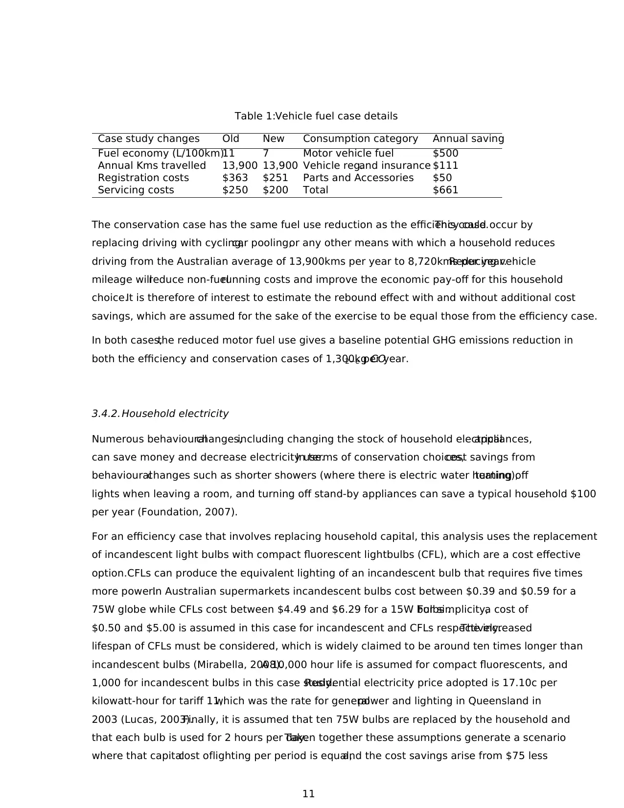
Table 1:Vehicle fuel case details
Case study changes Old New Consumption category Annual saving
Fuel economy (L/100km)11 7 Motor vehicle fuel $500
Annual Kms travelled 13,900 13,900 Vehicle reg.and insurance $111
Registration costs $363 $251 Parts and Accessories $50
Servicing costs $250 $200 Total $661
The conservation case has the same fuel use reduction as the efficiency case.This could occur by
replacing driving with cycling,car pooling,or any other means with which a household reduces
driving from the Australian average of 13,900kms per year to 8,720kms per year.Reducing vehicle
mileage willreduce non-fuelrunning costs and improve the economic pay-off for this household
choice.It is therefore of interest to estimate the rebound effect with and without additional cost
savings, which are assumed for the sake of the exercise to be equal those from the efficiency case.
In both cases,the reduced motor fuel use gives a baseline potential GHG emissions reduction in
both the efficiency and conservation cases of 1,300kg CO2−e per year.
3.4.2. Household electricity
Numerous behaviouralchanges,including changing the stock of household electricalappliances,
can save money and decrease electricity use.In terms of conservation choices,cost savings from
behaviouralchanges such as shorter showers (where there is electric water heating),turning off
lights when leaving a room, and turning off stand-by appliances can save a typical household $100
per year (Foundation, 2007).
For an efficiency case that involves replacing household capital, this analysis uses the replacement
of incandescent light bulbs with compact fluorescent lightbulbs (CFL), which are a cost effective
option.CFLs can produce the equivalent lighting of an incandescent bulb that requires five times
more power.In Australian supermarkets incandescent bulbs cost between $0.39 and $0.59 for a
75W globe while CFLs cost between $4.49 and $6.29 for a 15W bulbs .For simplicity,a cost of
$0.50 and $5.00 is assumed in this case for incandescent and CFLs respectively.The increased
lifespan of CFLs must be considered, which is widely claimed to be around ten times longer than
incandescent bulbs (Mirabella, 2008).A 10,000 hour life is assumed for compact fluorescents, and
1,000 for incandescent bulbs in this case study.Residential electricity price adopted is 17.10c per
kilowatt-hour for tariff 11,which was the rate for generalpower and lighting in Queensland in
2003 (Lucas, 2003).Finally, it is assumed that ten 75W bulbs are replaced by the household and
that each bulb is used for 2 hours per day.Taken together these assumptions generate a scenario
where that capitalcost oflighting per period is equal,and the cost savings arise from $75 less
11