Equilibrium Level of National Income Model

Runing head: MACROECONOMICS
Macroeconomics
Name of the Student
Name of the University
Course ID

1MACROECONOMICS
Table of Contents
Question 1..................................................................................................................................2
Question A.............................................................................................................................2
Question B..............................................................................................................................3
Question C..............................................................................................................................3
Question D.............................................................................................................................4
Question 2..................................................................................................................................5
Question A.............................................................................................................................5
Question B..............................................................................................................................6
Question C..............................................................................................................................7
Question D.............................................................................................................................8
Question 3..................................................................................................................................8
Question A.............................................................................................................................8
Question B..............................................................................................................................9
Question C............................................................................................................................10
Question D...........................................................................................................................12
References................................................................................................................................14

2MACROECONOMICS
Question 1
Question A
In the Keynesian model, national income in the short run is determined by aggregate
effective demand. The model was initially based upon two sectors consisting household and
business only. Later the model was extended for four sectors where aggregate demand or
aggregate expenditure is the sum of consumption expenditure, investment expenditure,
government expenditure and net earnings from foreign sector (Goodwin et al. 2015).
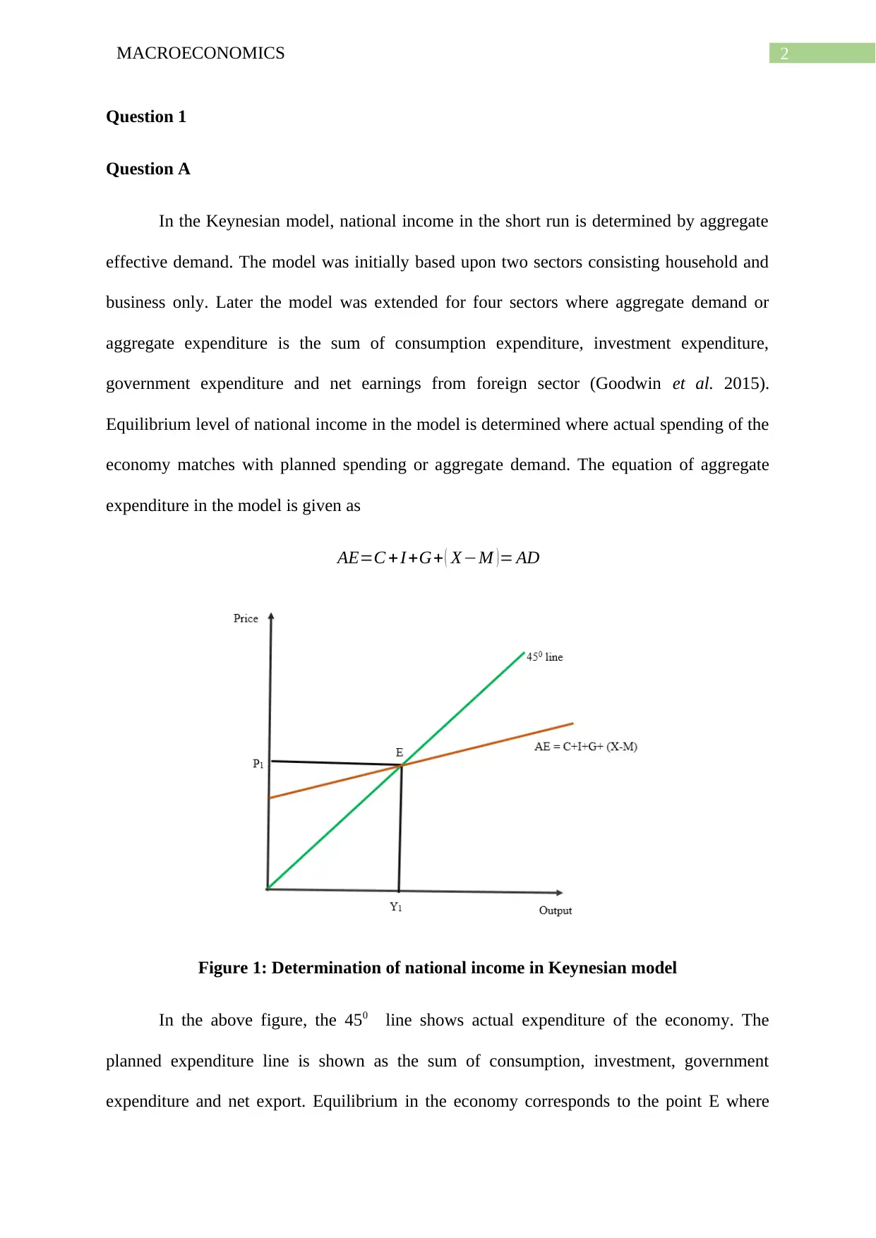
Equilibrium level of national income in the model is determined where actual spending of the
economy matches with planned spending or aggregate demand. The equation of aggregate
expenditure in the model is given as
AE=C + I +G+ ( X−M )= AD
Figure 1: Determination of national income in Keynesian model
In the above figure, the 450 line shows actual expenditure of the economy. The
planned expenditure line is shown as the sum of consumption, investment, government
expenditure and net export. Equilibrium in the economy corresponds to the point E where

3MACROECONOMICS
aggregate expenditure or demand matches actual expenditure or aggregate supply. Changes in
any component of aggregate spending results in a change in aggregate demand and an
associated change in national income.
Question B
An increase in saving rate is often considered to increase capital formation to increase
causing an increase in GDP. This however is not the case always. Income of a household is
generally divided between consumption and saving. A higher saving propensity actually leads
to a decline in consumption level and income without any increase in rather decrease in
aggregate saving of the economy. The impact of increase in saving propensity explained as
thriftiness of people on equilibrium income, consumption and saving is known as paradox of
thrift. According to Keynes a higher saving rate though is welcome from view of individual
household, it is not good from aggregate perspective since it has a damaging impact on
national income (Uribe and Schmitt-Grohe 2017). The reason for a fall in GDP because of an
increase in saving rate is given as higher saving rate means a lower propensity to consume.
As households consume less, there is a smaller demand for production causing a fall in
induced investment. Because of decline in factor employment there is a fall in income
generation resulting in a smaller GDP.
Question C
A low output and high unemployment rate indicates recessionary state of the
economy. In such a situation the economy needs necessary policy stimulus from the
government. One way to boost aggregate demand and expand output and employment is to
undertake expansionary fiscal policy by increasing spending. Government expenditure being
one important component of aggregate demand, as government spending increases there is an

4MACROECONOMICS
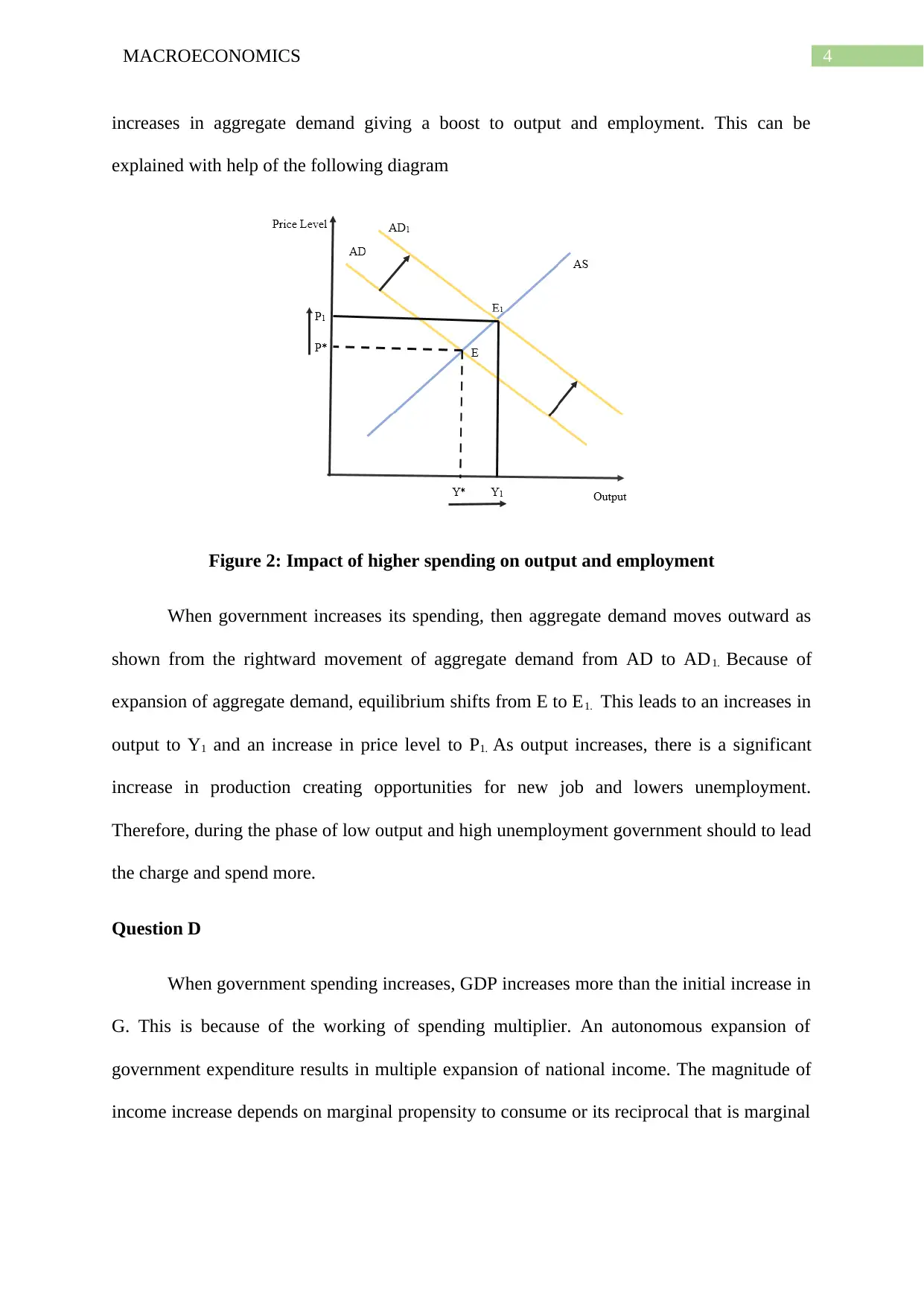
increases in aggregate demand giving a boost to output and employment. This can be
explained with help of the following diagram
Figure 2: Impact of higher spending on output and employment
When government increases its spending, then aggregate demand moves outward as
shown from the rightward movement of aggregate demand from AD to AD1. Because of
expansion of aggregate demand, equilibrium shifts from E to E1. This leads to an increases in
output to Y1 and an increase in price level to P1. As output increases, there is a significant
increase in production creating opportunities for new job and lowers unemployment.
Therefore, during the phase of low output and high unemployment government should to lead
the charge and spend more.
Question D
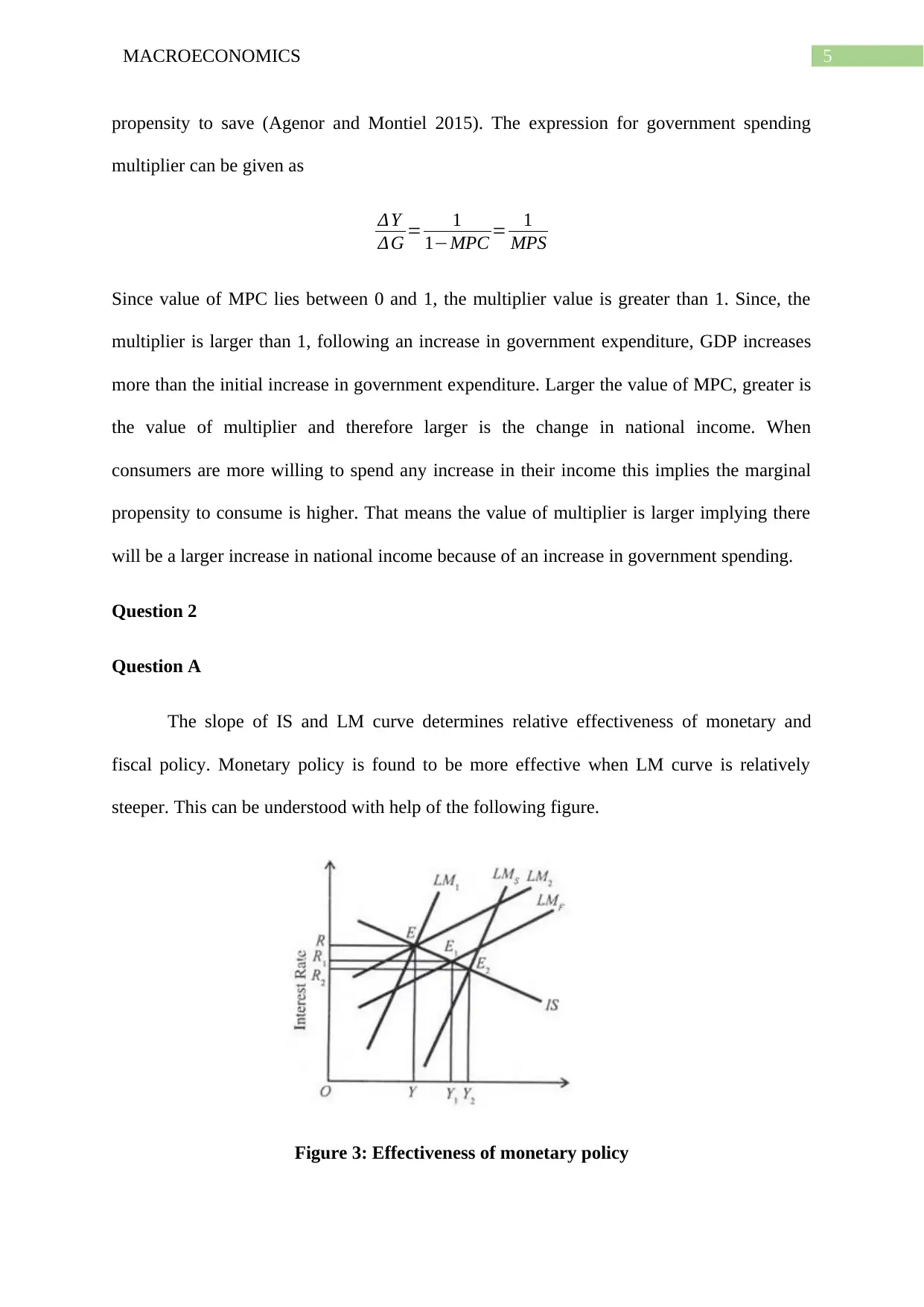
When government spending increases, GDP increases more than the initial increase in
G. This is because of the working of spending multiplier. An autonomous expansion of
government expenditure results in multiple expansion of national income. The magnitude of
income increase depends on marginal propensity to consume or its reciprocal that is marginal

5MACROECONOMICS
propensity to save (Agenor and Montiel 2015). The expression for government spending
multiplier can be given as
Δ Y
Δ G = 1
1−MPC = 1
MPS
Since value of MPC lies between 0 and 1, the multiplier value is greater than 1. Since, the
multiplier is larger than 1, following an increase in government expenditure, GDP increases
more than the initial increase in government expenditure. Larger the value of MPC, greater is
the value of multiplier and therefore larger is the change in national income. When
consumers are more willing to spend any increase in their income this implies the marginal
propensity to consume is higher. That means the value of multiplier is larger implying there
will be a larger increase in national income because of an increase in government spending.
Question 2
Question A
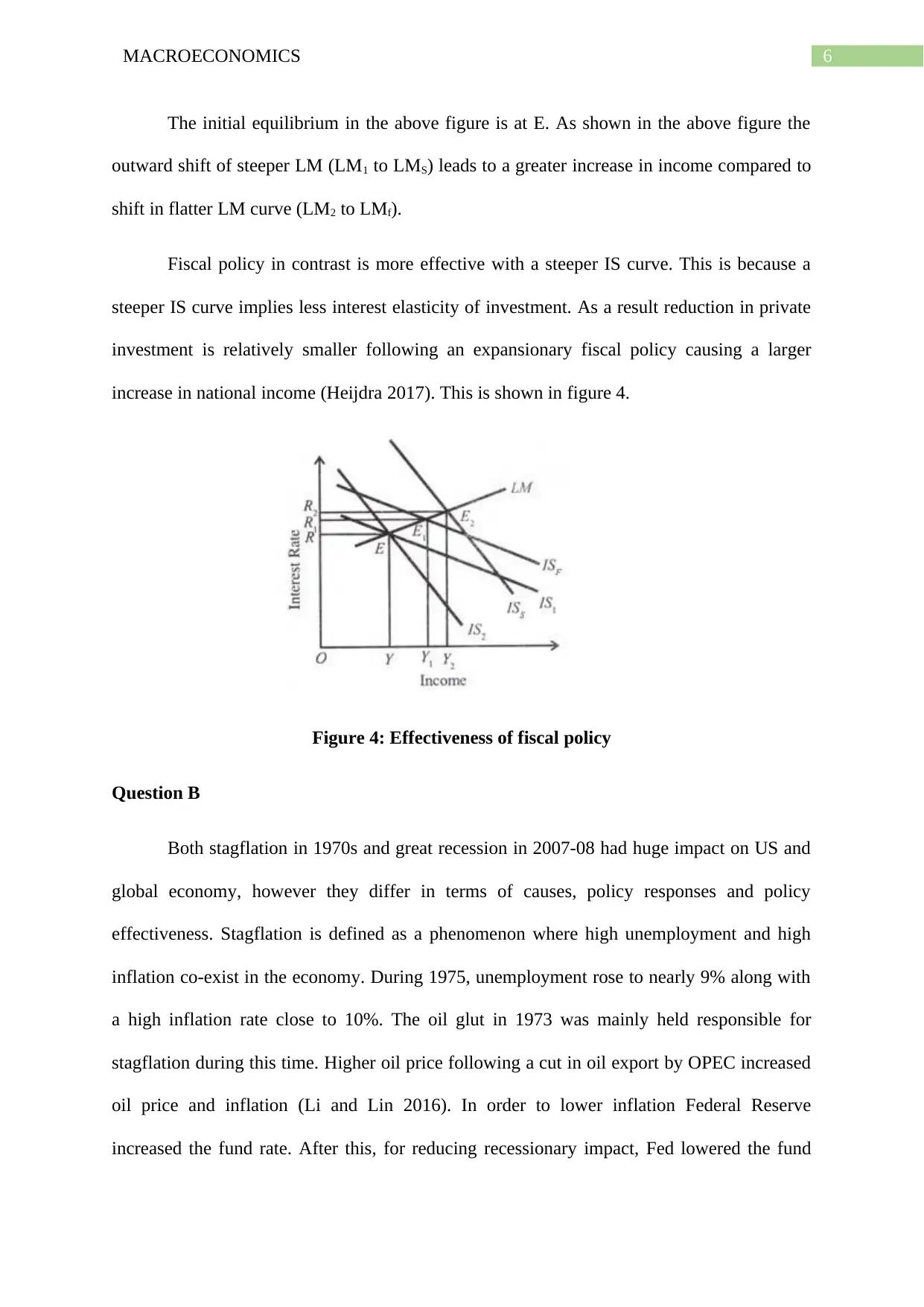
The slope of IS and LM curve determines relative effectiveness of monetary and
fiscal policy. Monetary policy is found to be more effective when LM curve is relatively
steeper. This can be understood with help of the following figure.
Figure 3: Effectiveness of monetary policy

6MACROECONOMICS
The initial equilibrium in the above figure is at E. As shown in the above figure the
outward shift of steeper LM (LM1 to LMS) leads to a greater increase in income compared to
shift in flatter LM curve (LM2 to LMf).
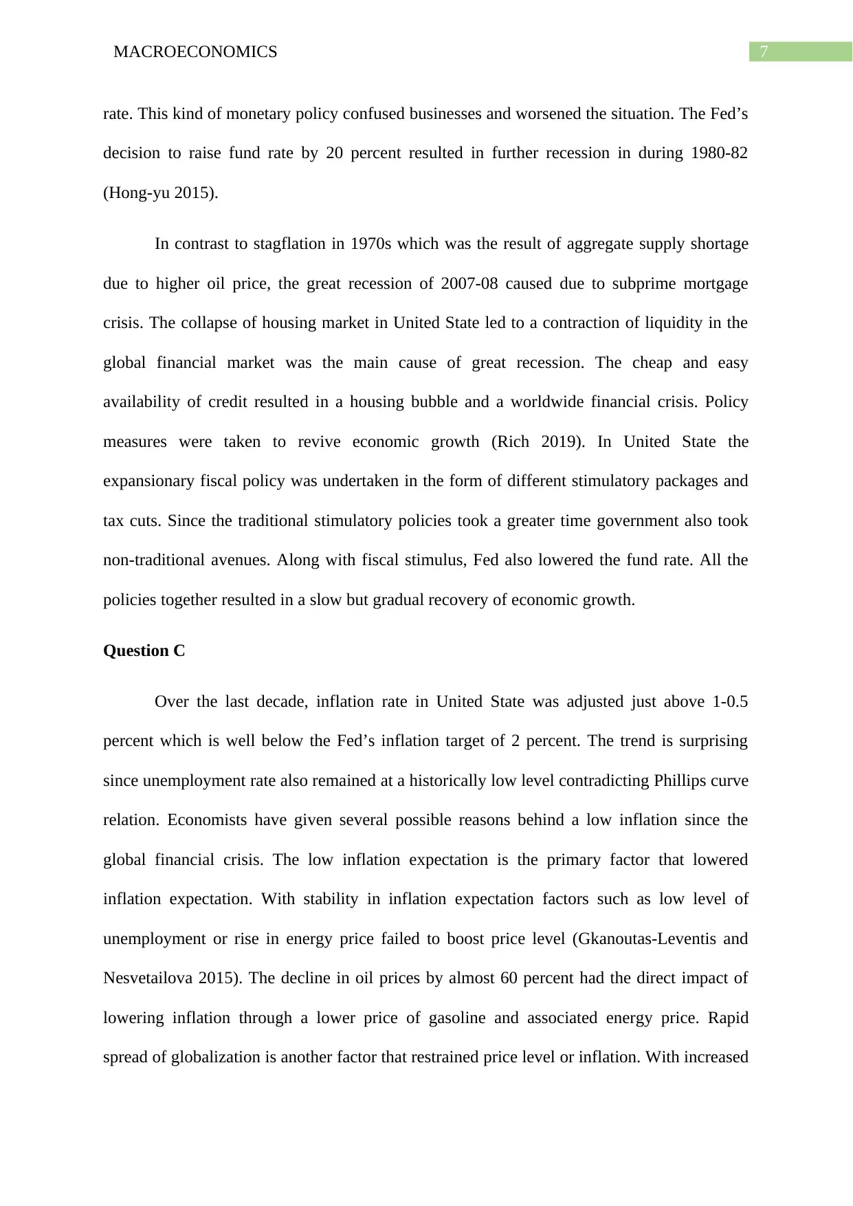
Fiscal policy in contrast is more effective with a steeper IS curve. This is because a
steeper IS curve implies less interest elasticity of investment. As a result reduction in private
investment is relatively smaller following an expansionary fiscal policy causing a larger
increase in national income (Heijdra 2017). This is shown in figure 4.
Figure 4: Effectiveness of fiscal policy
Question B
Both stagflation in 1970s and great recession in 2007-08 had huge impact on US and
global economy, however they differ in terms of causes, policy responses and policy
effectiveness. Stagflation is defined as a phenomenon where high unemployment and high
inflation co-exist in the economy. During 1975, unemployment rose to nearly 9% along with
a high inflation rate close to 10%. The oil glut in 1973 was mainly held responsible for
stagflation during this time. Higher oil price following a cut in oil export by OPEC increased
oil price and inflation (Li and Lin 2016). In order to lower inflation Federal Reserve
increased the fund rate. After this, for reducing recessionary impact, Fed lowered the fund

7MACROECONOMICS
rate. This kind of monetary policy confused businesses and worsened the situation. The Fed’s
decision to raise fund rate by 20 percent resulted in further recession in during 1980-82
(Hong-yu 2015).
In contrast to stagflation in 1970s which was the result of aggregate supply shortage
due to higher oil price, the great recession of 2007-08 caused due to subprime mortgage
crisis. The collapse of housing market in United State led to a contraction of liquidity in the
global financial market was the main cause of great recession. The cheap and easy
availability of credit resulted in a housing bubble and a worldwide financial crisis. Policy
measures were taken to revive economic growth (Rich 2019). In United State the
expansionary fiscal policy was undertaken in the form of different stimulatory packages and
tax cuts. Since the traditional stimulatory policies took a greater time government also took
non-traditional avenues. Along with fiscal stimulus, Fed also lowered the fund rate. All the
policies together resulted in a slow but gradual recovery of economic growth.
Question C
Over the last decade, inflation rate in United State was adjusted just above 1-0.5
percent which is well below the Fed’s inflation target of 2 percent. The trend is surprising
since unemployment rate also remained at a historically low level contradicting Phillips curve
relation. Economists have given several possible reasons behind a low inflation since the
global financial crisis. The low inflation expectation is the primary factor that lowered
inflation expectation. With stability in inflation expectation factors such as low level of
unemployment or rise in energy price failed to boost price level (Gkanoutas-Leventis and
Nesvetailova 2015). The decline in oil prices by almost 60 percent had the direct impact of
lowering inflation through a lower price of gasoline and associated energy price. Rapid
spread of globalization is another factor that restrained price level or inflation. With increased

8MACROECONOMICS
linkage among countries, inflation in US no longer determined by domestic factors. The
ongoing economic slow-down is one factor for core inflation to be low.
Given stability in inflation expectation, it is believed that inflation in United State will
pick up. Some of the forces holding down inflation has started to fade away. With a
diminishing state of labor market slack further downward pressure on labor market will be
diminished from this channel.
Question D
After the great recession during 2007-08, the economy experienced a significant
downfall. Contraction of economic activity during this time reduced labor demand
considerably pushing up the unemployment rate to the peak level of 10 percent. With
economic recovery unemployment though lowered it however took a relatively larger time
for unemployment to get back to pre-recession level (Orhangazi 2015). The main reason for
slow recovery of labor market was inadequate labor demand for a considerably long period.
Wage was also stagnated for working and middle class workers. Because of a very little
structural change in the economy causing inadequate labor demand.
The easing fiscal policy lower private investment through the crowding out effect.
With a high level of private investment there would have a faster expansion of private sectors
causing unemployment rate to fall faster. The ease fiscal policy further resulted in a deficit in
government budget resulting in a lack of funds for further employment opportunity.
Question 3
Question A
The stance of monetary policy is likely to be evaluated depending on a particular
variable or set of variables that are able to capture transmission mechanism of monetary

9MACROECONOMICS
policy. The variable particularly explaining stance of monetary policy is the short term
interest rate. If actual inflation rate overshoots the targeted rate, then Central bank increases
the interest rate to curb demand and inflation. This is called tight monetary policy. In
contrast, when inflation rate is below the central bank’s targeted rate, Central bank lowers the
interest rate to boost economic activity to push the price level up (Mankiw 2019). This is
known as ease or loose monetary policy. Monetary policy is said to be neutral when Central
bank neither increases nor decreases the interest rate. This happens when inflation rate is line
with targeted inflation rate.
Question B
Phillips curve as given by A.W. Phillips depicts an inverse relation between
unemployment and inflation rate. That is inflation increases with fall in unemployment and
vice-versa.
Because of the inverse relation between inflation and unemployment, Phillips curve
slopes downward. This is because during economic boom, labor demand increases resulting
in a fall in unemployment rate. A higher labor demand in turn increases bargaining power of
workers pushing up wage inflation.
A flatter Phillips curve implies that there is a relatively softer relation between wage
inflation and unemployment. This in turn suggests that unemployment rate can further be
reduced without upward pressure on price level.
A flat Phillips curve means a softer relation between output and price level implying a
steeper Aggregate Supply curve.
When Phillips curve is flatter the combination of output variability and inflation
become less favorable. The central bank therefore needs to generate a greater variability in
the domestic demand for achieving the desired inflation target. The softer relation between

10MACROECONOMICS
inflation and unemployment makes it easier for central bank to take policies to boost
employment since it does not increase inflationary pressure much.
Question C
The financial condition refers to state of different components related to overall
financial health of the economy. The four important components for analyzing financial
conditions are US dollar, corporate bonds spread, equity market level and level of interest in
different maturities.
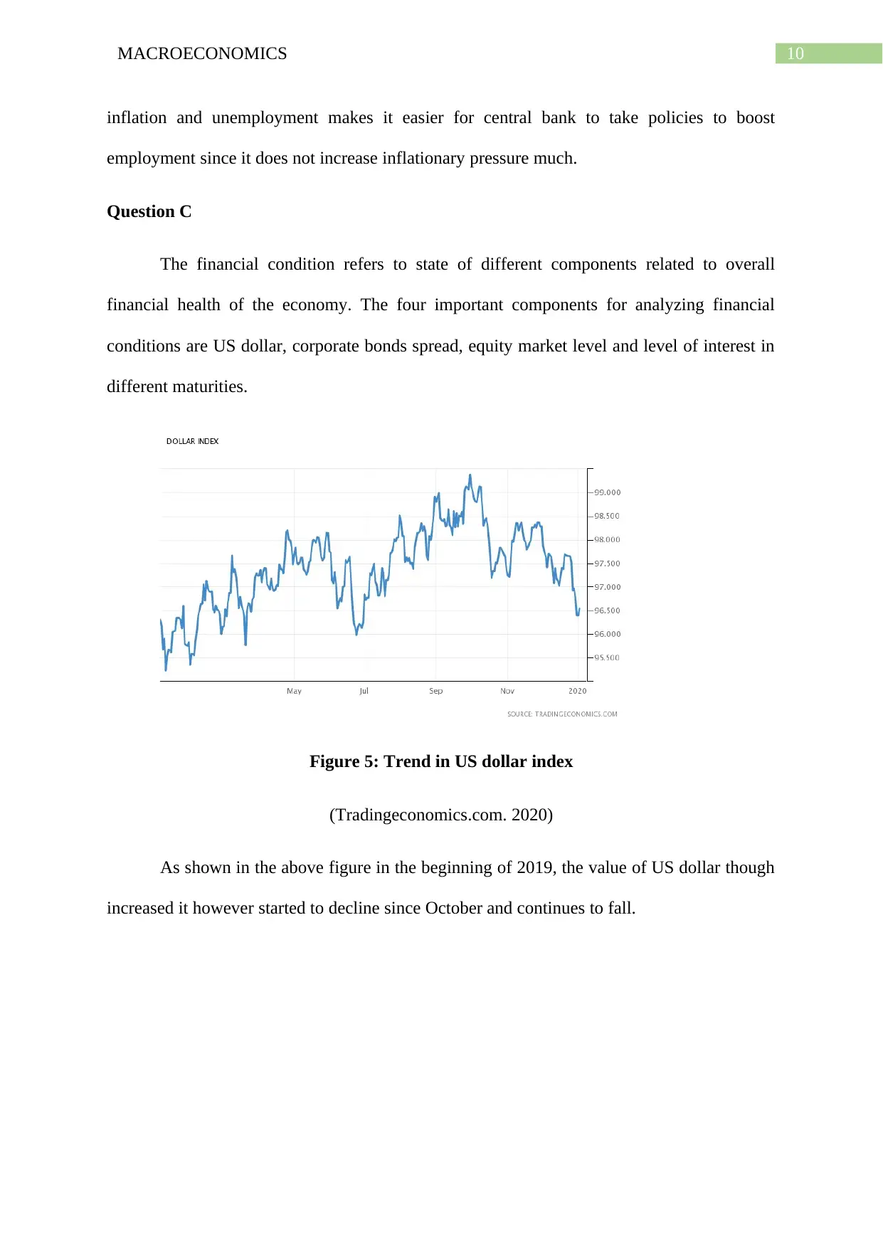
Figure 5: Trend in US dollar index
(Tradingeconomics.com. 2020)
As shown in the above figure in the beginning of 2019, the value of US dollar though
increased it however started to decline since October and continues to fall.

11MACROECONOMICS
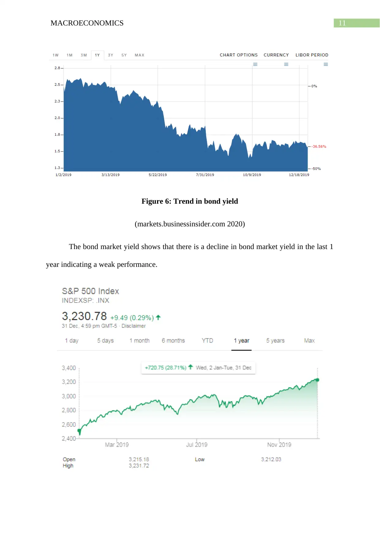
Figure 6: Trend in bond yield
(markets.businessinsider.com 2020)
The bond market yield shows that there is a decline in bond market yield in the last 1
year indicating a weak performance.

12MACROECONOMICS
Figure 7: Equity market performance
The performance of equity market shows a satisfactory performance with a gradual
increase in return.
Figure 8: Long term interest rate
(Ceicdata.com. 2020)
The Long term interest rate has declined significantly indicating a decline in return in
Treasury notes.
Financial condition has an important role in determining monetary policy. Stance of
monetary policy is commonly adjusted in line with financial conditions. The asset purchase
program as undertaken by central banks of aim at influencing the financial condition in the
risky asset markets which include sovereign debt market through term premium, mortgage
market and credit market. The rate of change in financial condition is an important
determinant of Fed’s monetary policy and interest rate decision.
Question D
Depending on financial condition of US in the last one and half year the market is
anticipating stronger economic growth. This in turn will help the investors to narrow down its

13MACROECONOMICS
focus on buying cyclical stocks (Domm 2019). The Fed’s officials in contrast is anticipating a
cut in interest rate because of uncertainties about economic growth. The uncertainties in the
broader global economy led Fed officials to doubt on stability of economic growth and that of
financial condition (Li 2019).
At present, inflation rate in United State is below the targeted level of 2 percent.
Along with this there is decline in global growth. Moreover the domestic economy is facing a
decline in business fixed investment (federalreserve.gov 2020). All these suggest the
economy needs a stimulus from government. Therefore, a Fed should take an ease monetary
policy to support the economy.

14MACROECONOMICS
References
Agenor, P.R. and Montiel, P.J., 2015. Development macroeconomics. Princeton University
Press.
Ceicdata.com. 2020. United States Long Term Interest Rate [1953 - 2020] [Data & Charts].
[online] Available at: https://www.ceicdata.com/en/indicator/united-states/long-term-
interest-rate [Accessed 2 Jan. 2020].
Domm, P. 2019. What the Fed's words say about how dovish it will be after a rate cut.
[online] CNBC. Available at: https://www.cnbc.com/2019/07/31/what-the-feds-
words-say-about-how-dovish-it-will-be-after-the-rate-cut.html [Accessed 2 Jan.
2020].
federalreserve.gov 2020. The Fed - Monetary Policy: . [online] Available at:
https://www.federalreserve.gov/monetarypolicy/fomcminutes20190918ep.htm
[Accessed 2 Jan. 2020].
Gkanoutas-Leventis, A. and Nesvetailova, A., 2015. Financialisation, oil and the Great
Recession. Energy policy, 86, pp.891-902.
Goodwin, N., Harris, J.M., Nelson, J.A., Roach, B. and Torras, M., 2015. Macroeconomics in
context. Routledge.
Heijdra, B.J., 2017. Foundations of modern macroeconomics. Oxford university press.
Hong-yu, Z.H.A.N.G., 2015. New Inquiry into Internal Cause of Stagflation in the United
States in the 1970s. Journal of Xuchang University, (1), p.23.
Li, J.F. and Lin, Z.X., 2016. Social benefit expenditures and stagflation: evidence from the
United States. Applied Economics, 48(55), pp.5340-5347.

15MACROECONOMICS
Li, Y. (2019). Goldman sees the economy surprising in 2020 and these stocks benefiting most
from the rebound. [online] CNBC. Available at:
https://www.cnbc.com/2019/11/18/goldman-sees-economy-surprising-in-2020-and-
these-stocks-will-benefit.html [Accessed 2 Jan. 2020].
Mankiw, N.G., 2019. Principles of macroeconomics. Cengage Learning.
markets.businessinsider.com 2020. U.S. Rates 2 Years Rates | Markets Insider. [online]
markets.businessinsider.com. Available at:
https://markets.businessinsider.com/rates/u-s--rates-2-years [Accessed 2 Jan. 2020].
Orhangazi, Ö., 2015. Financial deregulation and the 2007–08 US financial crisis. In The
Demise of Finance-dominated Capitalism. Edward Elgar Publishing.
Rich, R. 2019. The Great Recession | Federal Reserve History. [online]
Federalreservehistory.org. Available at:
https://www.federalreservehistory.org/essays/great_recession_of_200709 [Accessed 2
Jan. 2020].
Tradingeconomics.com. 2020. United States Dollar . [online] Available at:
https://tradingeconomics.com/united-states/currency [Accessed 2 Jan. 2020].
Uribe, M. and Schmitt-Grohe, S., 2017. Open economy macroeconomics. Princeton
University Press.