Profit Maximization and Monopoly Strategies for Suckers Corporation

The assignment content discusses the profit-maximizing strategy of Suckers Corporation, a company that produces portable vacuum cleaners. The table shows that by offering different quantities to customers in various weeks, the corporation can maximize its profit level. The report concludes that the equilibrium position is when marginal cost (MC) cuts marginal revenue (MR), and that people prefer to purchase products when price levels move in a decreasing way. It also suggests that the company can raise demand for its product by controlling its cost levels and offering it at a suitable price.

Economics

Table of Contents
INTRODUCTION......................................................................................................................3
1. Presenting a short run equilibrium of profit maximizing in short-run related to
monopolistic situation............................................................................................................3
2. Establishing relationship between demand and selling price.............................................4
a. Constructing cost and revenue and table............................................................................6
b..............................................................................................................................................7
1. Assessing profit maximizing level for output (each week)................................................7
2. Assessing profit maximizing price.....................................................................................8
3. Identifying maximum profit level......................................................................................8
CONCUSION............................................................................................................................9
REFERENCES.........................................................................................................................10
Figure 1: Short \-run equilibrium position.................................................................................3
Figure 2: Long-run equilibrium position....................................................................................4
Figure 3: Relationship between price and quantity demanded..................................................6
Figure 4: Cost curve...................................................................................................................8

INTRODUCTION
Field of economics is highly significant which in turn helps company in making
suitable decisions that directly aid in the growth and profitability aspect. It assists analyst in
making proper estimation of demand as well as supply and thereby helps in making suitable
pricing decisions. In this, report will develop understanding about short and long run
equilibrium position of monopolist. Further, it will also shed light on the extent to which
relationship takes place between sales and quantity demanded.
1. Presenting a short run equilibrium of profit maximizing in short-run related to
monopolistic situation
In the monopoly market, business unit can maximize profit level and reduce loss by
equalizing marginal cost and revenue. Business entity has opportunity to attain super or
normal in short run by performing activities in monopoly market (Elsadany and Awad, 2016).
Monopolists require satisfying the following aspects to get equilibrium position is as follows:
 First situation: Marginal cost (MC) = Marginal revenue (MR)
 Second situation: Equilibrium is when MC curve cuts MR (Monopoly diagram in long
and short run, 2016)
Equilibrium position with positive profit in short run is enumerated below:

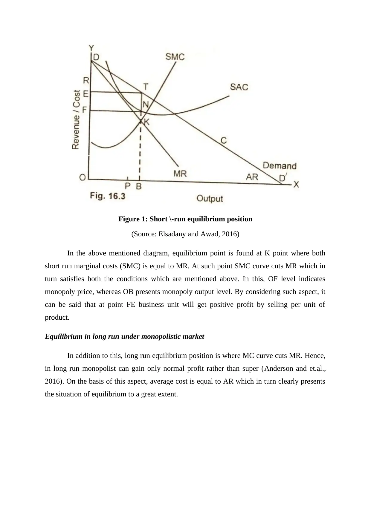
Figure 1: Short \-run equilibrium position
(Source: Elsadany and Awad, 2016)
In the above mentioned diagram, equilibrium point is found at K point where both
short run marginal costs (SMC) is equal to MR. At such point SMC curve cuts MR which in
turn satisfies both the conditions which are mentioned above. In this, OF level indicates
monopoly price, whereas OB presents monopoly output level. By considering such aspect, it
can be said that at point FE business unit will get positive profit by selling per unit of
product.
Equilibrium in long run under monopolistic market
In addition to this, long run equilibrium position is where MC curve cuts MR. Hence,
in long run monopolist can gain only normal profit rather than super (Anderson and et.al.,
2016). On the basis of this aspect, average cost is equal to AR which in turn clearly presents
the situation of equilibrium to a great extent.

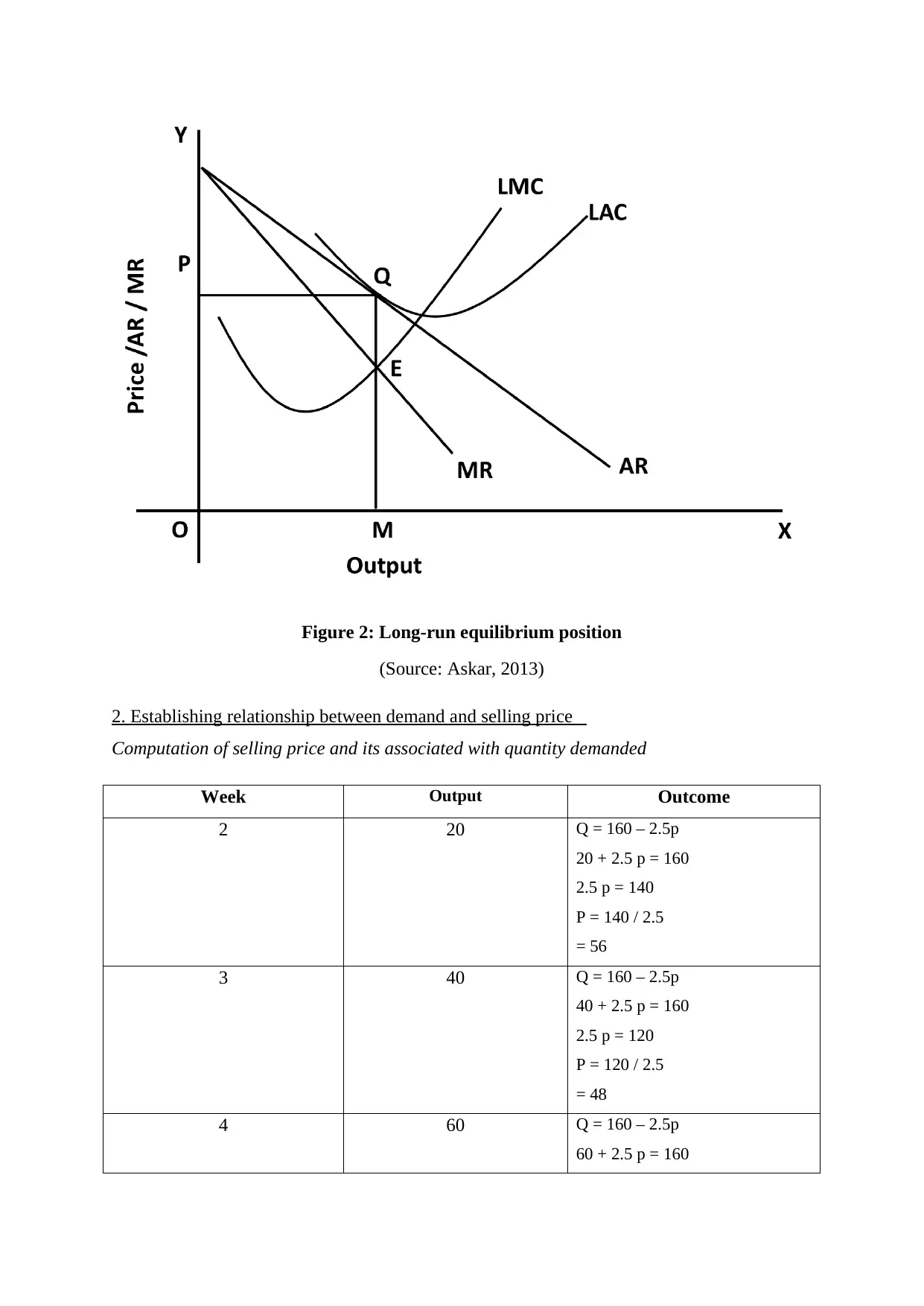
Figure 2: Long-run equilibrium position
(Source: Askar, 2013)
2. Establishing relationship between demand and selling price
Computation of selling price and its associated with quantity demanded
Week Output Outcome
2 20 Q = 160 – 2.5p
20 + 2.5 p = 160
2.5 p = 140
P = 140 / 2.5
= 56
3 40 Q = 160 – 2.5p
40 + 2.5 p = 160
2.5 p = 120
P = 120 / 2.5
= 48
4 60 Q = 160 – 2.5p
60 + 2.5 p = 160

2.5 p = 100
P = 100 / 2.5
= 40
5 80 Q = 160 – 2.5p
80 + 2.5 p = 160
2.5 p = 80
P = 80 / 2.5
= 32
6 100 Q = 160 – 2.5p
100 + 2.5 p = 160
2.5 p = 60
P = 60 / 2.5
= 24
1 2 3 4 5
0
20
40
60
80
100
120
Qauntity demanded
Price
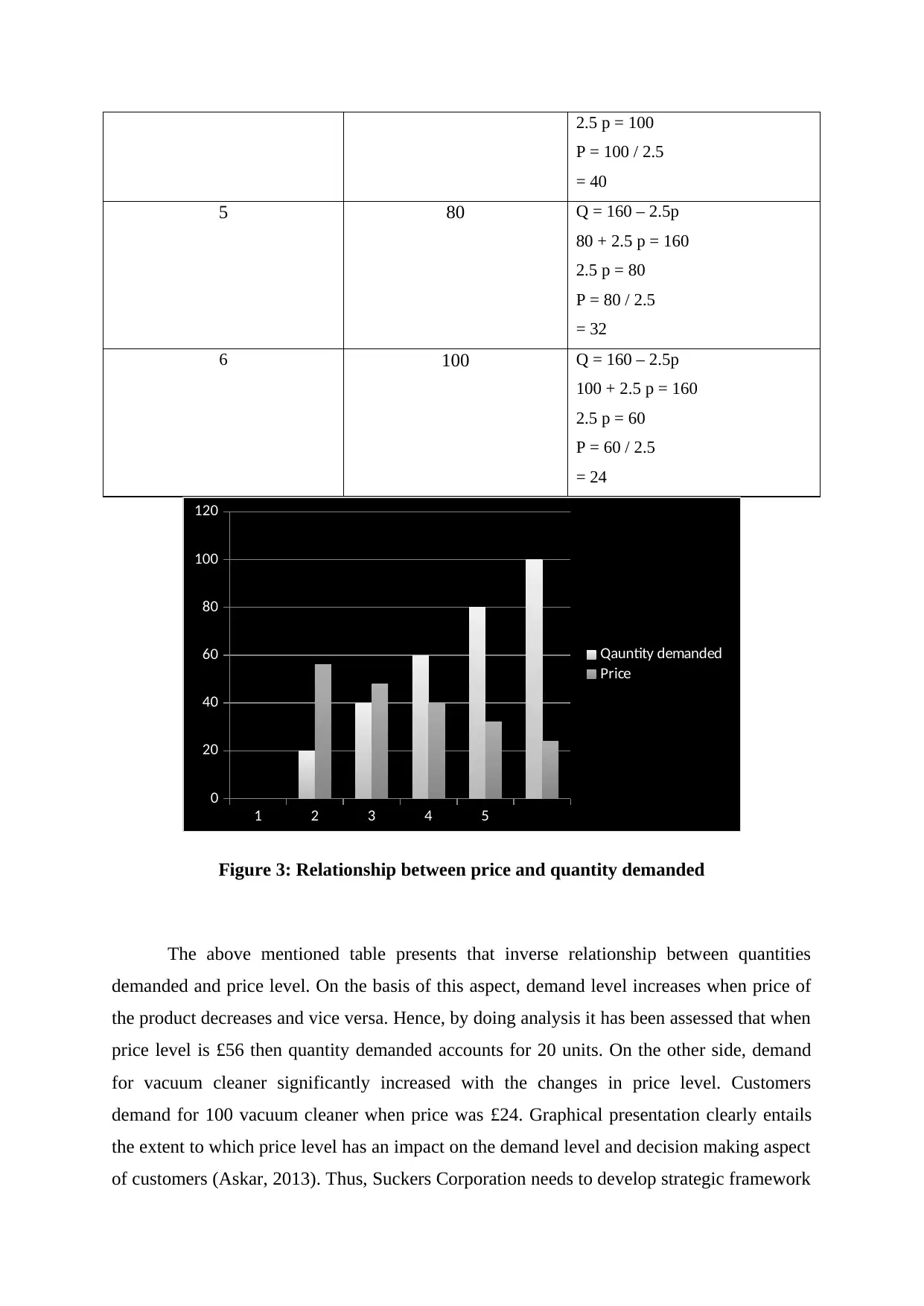
Figure 3: Relationship between price and quantity demanded
The above mentioned table presents that inverse relationship between quantities
demanded and price level. On the basis of this aspect, demand level increases when price of
the product decreases and vice versa. Hence, by doing analysis it has been assessed that when
price level is £56 then quantity demanded accounts for 20 units. On the other side, demand
for vacuum cleaner significantly increased with the changes in price level. Customers
demand for 100 vacuum cleaner when price was £24. Graphical presentation clearly entails
the extent to which price level has an impact on the demand level and decision making aspect
of customers (Askar, 2013). Thus, Suckers Corporation needs to develop strategic framework

by taking into consideration such trend. This in turn helps company in attracting the large
number of customers and thereby assists in fulfilling objectives.
a. Constructing cost and revenue and table
 Total variable cost: It implies for the cost which is incurred by business organization
to carry out business operations and function smoothly. Such cost is not directly
attributable to production object but include sales and administration expenses,
miscellaneous expenses etc (Ito, 2014). Marginal cost (MC): This method helps in assessing the change which will take place
in cost level on the production of one additional unit (Marginal revenue and cost,
2016). Hence, by using the following formula Suckers Corporation can assess
marginal cost is :
MC = ∆TC / ∆Output
 Average revenue (AR): This measure helps business entity in getting information
about revenue which is generated by firm from individual customer (Hirschey, 2016).
Formula of average revenue is enumerated below:
AR = P
AR = (Price * quantity) / quantity
 Marginal revenue (MR): By employing such measure business unit can assess the
revenue gained by it from one additional unit of output (Delis, Iosifidi and Tsionas,
2014). Hence, by considering such measure company can take suitable decision about
production or output level.
MR = ∆TC / ∆Output
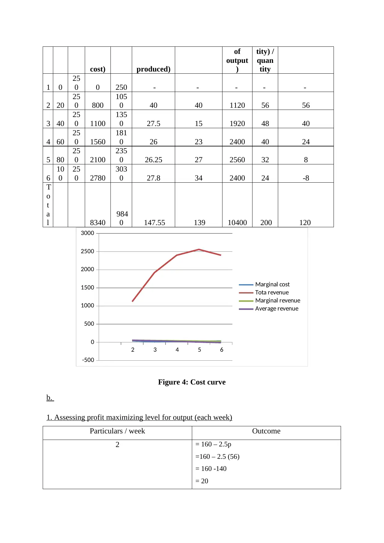
Computation of total variable, marginal cost, average and marginal revenue
w
e
e
k
O
ut
p
ut
Fi
xe
d
co
st
Vari
able
cost
(Tota
l cost
–
fixed
Tot
al
cost
Variable
cost per
unit
(Variable
cost /
number of
unit
Marginal
cost
(Changes in
total cost /
change in
output
level)
Total
revenu
e
(price
per
unit *
level
Aver
age
reven
ue
(Pric
e *
quan
Marginal
revenue
(change in
total revenue /
change in level
of output)

cost) produced)
of
output
)
tity) /
quan
tity
1 0
25
0 0 250 - - - - -
2 20
25
0 800
105
0 40 40 1120 56 56
3 40
25
0 1100
135
0 27.5 15 1920 48 40
4 60
25
0 1560
181
0 26 23 2400 40 24
5 80
25
0 2100
235
0 26.25 27 2560 32 8
6
10
0
25
0 2780
303
0 27.8 34 2400 24 -8
T
o
t
a
l 8340
984
0 147.55 139 10400 200 120
2 3 4 5 6
-500
0
500
1000
1500
2000
2500
3000
Marginal cost
Tota revenue
Marginal revenue
Average revenue
Figure 4: Cost curve
b.
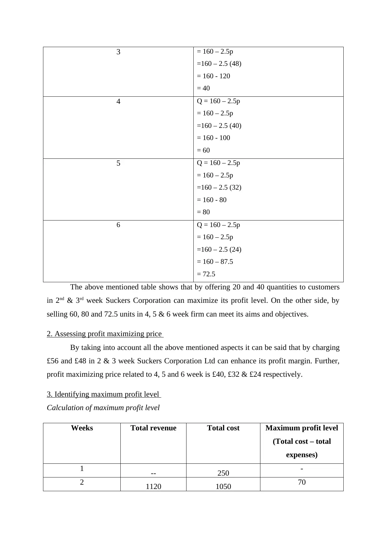
1. Assessing profit maximizing level for output (each week)
Particulars / week Outcome
2 = 160 – 2.5p
=160 – 2.5 (56)
= 160 -140
= 20

3 = 160 – 2.5p
=160 – 2.5 (48)
= 160 - 120
= 40
4 Q = 160 – 2.5p
= 160 – 2.5p
=160 – 2.5 (40)
= 160 - 100
= 60
5 Q = 160 – 2.5p
= 160 – 2.5p
=160 – 2.5 (32)
= 160 - 80
= 80
6 Q = 160 – 2.5p
= 160 – 2.5p
=160 – 2.5 (24)
= 160 – 87.5
= 72.5
The above mentioned table shows that by offering 20 and 40 quantities to customers
in 2nd & 3rd week Suckers Corporation can maximize its profit level. On the other side, by
selling 60, 80 and 72.5 units in 4, 5 & 6 week firm can meet its aims and objectives.
2. Assessing profit maximizing price
By taking into account all the above mentioned aspects it can be said that by charging
£56 and £48 in 2 & 3 week Suckers Corporation Ltd can enhance its profit margin. Further,
profit maximizing price related to 4, 5 and 6 week is £40, £32 & £24 respectively.
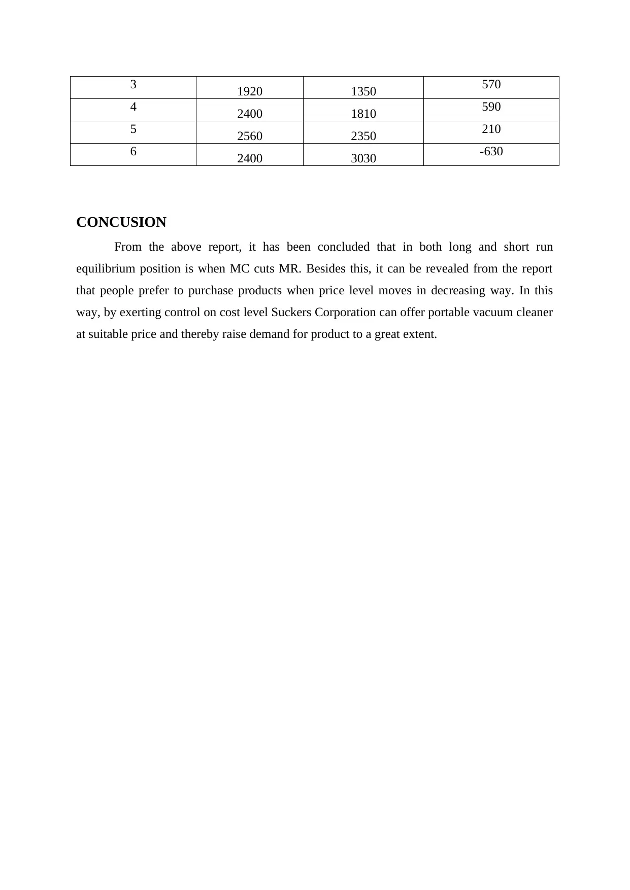
3. Identifying maximum profit level
Calculation of maximum profit level
Weeks Total revenue Total cost Maximum profit level
(Total cost – total
expenses)
1 -- 250 -
2 1120 1050 70

3 1920 1350 570
4 2400 1810 590
5 2560 2350 210
6 2400 3030 -630
CONCUSION
From the above report, it has been concluded that in both long and short run
equilibrium position is when MC cuts MR. Besides this, it can be revealed from the report
that people prefer to purchase products when price level moves in decreasing way. In this
way, by exerting control on cost level Suckers Corporation can offer portable vacuum cleaner
at suitable price and thereby raise demand for product to a great extent.